06. Visualizing and using sensitivities

One traced ray can say more than where the ray goes and when it arrives. LayTracer can also report how its travel time and physical ray parameter respond to small changes in the model and acquisition geometry.

This example traces a P wave that reflects as SV. The downgoing and upgoing legs therefore sample different velocity fields, giving one compact example with non-zero derivatives for \(V_P\), \(V_S\), interface depths, and the source and receiver coordinates.

Trace one selected ray

The source and receiver are 200 m deep. The selected wave travels down as P, reflects at 2500 m, and returns as SV. Requesting sensitivities and diagnostics is opt-in; the ordinary travel-time API is unchanged.

import time

import matplotlib.pyplot as plt
from matplotlib.lines import Line2D
import numpy as np
import pandas as pd

import laytracer as lt


# sphinx_gallery_thumbnail_number = 1

model = pd.DataFrame({
    "Depth": [0.0, 1200.0, 2500.0],
    "Vp": [2400.0, 3600.0, 5200.0],
    "Vs": [1350.0, 2050.0, 3000.0],
})
source = np.array([0.0, 0.0, 200.0])
receiver = np.array([4000.0, 0.0, 200.0])


def trace_ps_reflection(model_to_trace, source_to_trace, receiver_to_trace, requested):
    """Trace the selected P-down, SV-up reflection."""
    reflector_depth = float(model_to_trace.iloc[2]["Depth"])
    itinerary = lt.RayItinerary(
        source_phase="P",
        interactions=[lt.Interaction(reflector_depth, "reflect", "SV")],
    )
    return lt.trace_rays(
        source_to_trace,
        receiver_to_trace,
        model_to_trace,
        itinerary=itinerary,
        requested=requested,
        n_jobs=1,
        verbose=False,
        tol=1e-10,
        max_iter=30,
    )


reference = trace_ps_reflection(
    model,
    source,
    receiver,
    {"travel_times", "rays", "ray_parameters", "diagnostics", "sensitivities"},
)
diagnostic = reference.diagnostics[0]
sensitivity = reference.sensitivities[0]

assert diagnostic.converged
assert sensitivity.valid
np.testing.assert_array_equal(sensitivity.vp_layer_indices, [0, 1])
np.testing.assert_array_equal(sensitivity.vs_layer_indices, [0, 1])
np.testing.assert_array_equal(sensitivity.interface_indices, [1, 2])
assert sensitivity.dtravel_time_dsource[1] == 0.0
assert sensitivity.dtravel_time_dreceiver[1] == 0.0

print(f"Travel time: {reference.travel_times[0]:.4f} s")
print(f"Physical ray parameter p: {1e6 * reference.ray_parameters[0]:.3f} us/m")
print(
    f"Solve: {diagnostic.method}, endpoint residual "
    f"{diagnostic.absolute_offset_residual:.2e} m"
)
print("Vp layer indices:", sensitivity.vp_layer_indices)
print("dT/dVp:", sensitivity.dtravel_time_dvp)
print("dp/dVp:", sensitivity.dray_parameter_dvp)
print("Vs layer indices:", sensitivity.vs_layer_indices)
print("dT/dVs:", sensitivity.dtravel_time_dvs)
print("dp/dVs:", sensitivity.dray_parameter_dvs)
print("Interface indices:", sensitivity.interface_indices)
print("dT/dz_interface:", sensitivity.dtravel_time_dinterface_depths)
print("dp/dz_interface:", sensitivity.dray_parameter_dinterface_depths)
print("dT/dsource:", sensitivity.dtravel_time_dsource)
print("dp/dsource:", sensitivity.dray_parameter_dsource)
print("dT/dreceiver:", sensitivity.dtravel_time_dreceiver)
print("dp/dreceiver:", sensitivity.dray_parameter_dreceiver)

Travel time: 2.7353 s
Physical ray parameter p: 239.729 us/m
Solve: q_newton, endpoint residual 0.00e+00 m
Vp layer indices: [0 1]
dT/dVp: [-0.00021226 -0.00019857]
dp/dVp: [-9.45918613e-09 -5.21938605e-08]
Vs layer indices: [0 1]
dT/dVs: [-0.00057991 -0.00035519]
dp/dVs: [-6.11000692e-09 -1.01857138e-08]
Interface indices: [1 2]
dT/dz_interface: [0.00047651 0.00056516]
dp/dz_interface: [ 2.64952412e-08 -4.90668503e-08]
dT/dsource: [-0.00023973 -0.         -0.00034079]
dp/dsource: [-2.15896286e-08 -0.00000000e+00  1.51870421e-08]
dT/dreceiver: [ 0.00023973  0.         -0.00070088]
dp/dreceiver: [2.15896286e-08 0.00000000e+00 7.38456700e-09]

Visualize the sensitivity fingerprint

Raw derivatives have different units, so plotting them together would be misleading. Instead, apply small, clearly labelled changes: 1% to a velocity and 10 m to an interface or endpoint. Each derivative then becomes a predicted travel-time shift in milliseconds and a physical-ray-parameter shift in microseconds per metre.

effect_rows = []

for layer_index, dtime, dparameter in zip(
    sensitivity.vp_layer_indices,
    sensitivity.dtravel_time_dvp,
    sensitivity.dray_parameter_dvp,
):
    change = 0.01 * model.loc[layer_index, "Vp"]
    effect_rows.append((
        rf"$V_P$ layer {layer_index + 1} (+1%)",
        "P velocity",
        dtime * change,
        dparameter * change,
    ))

for layer_index, dtime, dparameter in zip(
    sensitivity.vs_layer_indices,
    sensitivity.dtravel_time_dvs,
    sensitivity.dray_parameter_dvs,
):
    change = 0.01 * model.loc[layer_index, "Vs"]
    effect_rows.append((
        rf"$V_S$ layer {layer_index + 1} (+1%)",
        "S velocity",
        dtime * change,
        dparameter * change,
    ))

for interface_index, dtime, dparameter in zip(
    sensitivity.interface_indices,
    sensitivity.dtravel_time_dinterface_depths,
    sensitivity.dray_parameter_dinterface_depths,
):
    label = "reflector" if interface_index == 2 else "interface 1"
    effect_rows.append((
        f"{label} deeper (+10 m)",
        "Interface",
        dtime * 10.0,
        dparameter * 10.0,
    ))

endpoint_changes = (
    ("source right (+10 m)", "Source", sensitivity.dtravel_time_dsource[0], sensitivity.dray_parameter_dsource[0]),
    ("source deeper (+10 m)", "Source", sensitivity.dtravel_time_dsource[2], sensitivity.dray_parameter_dsource[2]),
    ("receiver right (+10 m)", "Receiver", sensitivity.dtravel_time_dreceiver[0], sensitivity.dray_parameter_dreceiver[0]),
    ("receiver deeper (+10 m)", "Receiver", sensitivity.dtravel_time_dreceiver[2], sensitivity.dray_parameter_dreceiver[2]),
)
for label, group, dtime, dparameter in endpoint_changes:
    effect_rows.append((label, group, dtime * 10.0, dparameter * 10.0))

effects = pd.DataFrame(
    effect_rows,
    columns=["change", "group", "delta_time_s", "delta_parameter_s_per_m"],
)
effects["delta_time_ms"] = 1e3 * effects["delta_time_s"]
effects["delta_parameter_us_per_m"] = 1e6 * effects["delta_parameter_s_per_m"]

print("\nSensitivity fingerprint for the labelled changes:")
print(effects[["change", "delta_time_ms", "delta_parameter_us_per_m"]].to_string(index=False))

# Move only the reflector for the dashed comparison ray.
deeper_model = model.copy()
deeper_model.loc[2, "Depth"] += 100.0
deeper = trace_ps_reflection(
    deeper_model,
    source,
    receiver,
    {"travel_times", "rays", "ray_parameters"},
)

group_colors = {
    "P velocity": "#0072B2",
    "S velocity": "#CC79A7",
    "Interface": "#009E73",
    "Source": "#E69F00",
    "Receiver": "#6B6B6B",
}
colors = [group_colors[group] for group in effects["group"]]

figure = plt.figure(figsize=(12.8, 13.0))
grid = figure.add_gridspec(2, 2, height_ratios=[3.0, 1.0])
axes = [
    figure.add_subplot(grid[0, :]),
    figure.add_subplot(grid[1, 0]),
    figure.add_subplot(grid[1, 1]),
]

axis = axes[0]
axis.axhspan(0.0, 1.2, color="#DCEAF4")
axis.axhspan(1.2, 2.5, color="#B7D5E8")
axis.axhspan(2.5, 2.9, color="#E9ECEF")
axis.axhline(1.2, color="white", linewidth=1.4)
axis.axhline(2.5, color="#009E73", linewidth=1.3)
axis.axhline(2.6, color="#009E73", linewidth=1.3, linestyle="--")

ray = reference.rays[0]
turning_index = int(np.argmax(ray[:, 2]))
axis.plot(ray[: turning_index + 1, 0] / 1000.0, ray[: turning_index + 1, 2] / 1000.0, color="#0072B2", linewidth=2.5)
axis.plot(ray[turning_index:, 0] / 1000.0, ray[turning_index:, 2] / 1000.0, color="#CC79A7", linewidth=2.5)
perturbed_ray = deeper.rays[0]
axis.plot(perturbed_ray[:, 0] / 1000.0, perturbed_ray[:, 2] / 1000.0, color="#333333", linewidth=1.3, linestyle="--", alpha=0.8)
axis.scatter(source[0] / 1000.0, source[2] / 1000.0, marker="*", s=90, color="#222222", zorder=5)
axis.scatter(receiver[0] / 1000.0, receiver[2] / 1000.0, marker="v", s=55, color="#222222", zorder=5)
axis.text(0.12, 0.78, "layer 1", transform=axis.transAxes, color="#354F60")
axis.text(0.12, 0.47, "layer 2", transform=axis.transAxes, color="#354F60")
axis.text(2.65, 2.78, "layer below reflector\n(not sampled)", ha="center", color="#6B6B6B", fontsize=8)
axis.text(0.58, 1.02, "P", color="#0072B2", fontweight="bold")
axis.text(3.55, 0.72, "SV", color="#CC79A7", fontweight="bold")
axis.text(0.12, 2.47, "reference reflector", color="#007C5B", va="bottom", fontsize=8)
axis.text(0.12, 2.67, "reflector +100 m", color="#007C5B", va="top", fontsize=8)
axis.text(
    0.52,
    0.965,
    "$\\Delta T$: arrival shift     $\\Delta p$: launch-direction shift",
    transform=axis.transAxes,
    ha="center",
    va="top",
    fontsize=8.0,
    bbox={"boxstyle": "round,pad=0.35", "facecolor": "white", "alpha": 0.88, "edgecolor": "#BBBBBB"},
)
axis.set_xlim(-0.15, 4.15)
axis.set_ylim(2.9, 0.0)
axis.set_aspect("equal", adjustable="box")
axis.set_xlabel("Horizontal distance (km)")
axis.set_ylabel("Depth (km)")
axis.set_title("(a) One selected P-to-SV reflection")


def sensitivity_lollipops(axis, values, xlabel, title):
    """Draw one signed, annotated sensitivity-effect chart."""
    positions = np.arange(len(effects))
    limit = 1.28 * np.max(np.abs(values))
    axis.axvline(0.0, color="#444444", linewidth=0.8)
    axis.hlines(positions, 0.0, values, colors=colors, linewidth=2.0)
    axis.scatter(values, positions, c=colors, s=43, zorder=3)
    for position, value in zip(positions, values):
        offset = 0.025 * limit if value >= 0.0 else -0.025 * limit
        axis.text(
            value + offset,
            position,
            f"{value:+.2f}",
            va="center",
            ha="left" if value >= 0.0 else "right",
            fontsize=7.4,
        )
    axis.set_xlim(-limit, limit)
    axis.set_ylim(len(effects) - 0.35, -0.65)
    axis.set_yticks(positions, effects["change"])
    axis.set_xlabel(xlabel)
    axis.set_title(title)
    axis.grid(axis="x", alpha=0.22)


sensitivity_lollipops(
    axes[1],
    effects["delta_time_ms"].to_numpy(),
    "Predicted arrival-time change (ms)",
    "(b) What moves the arrival time?",
)
sensitivity_lollipops(
    axes[2],
    effects["delta_parameter_us_per_m"].to_numpy(),
    r"Predicted change in physical $p$ ($\mu$s/m)",
    "(c) What steers the ray?",
)
axes[2].set_yticklabels([])

legend_handles = [
    Line2D([0], [0], marker="o", linestyle="", color=color, label=group)
    for group, color in group_colors.items()
]
figure.legend(handles=legend_handles, frameon=False, ncol=5, loc="lower center", bbox_to_anchor=(0.5, 0.01))
figure.suptitle("What changes this arrival?", fontsize=14)
figure.subplots_adjust(left=0.17, right=0.97, top=0.93, bottom=0.10, hspace=0.35, wspace=0.25)
plt.show()

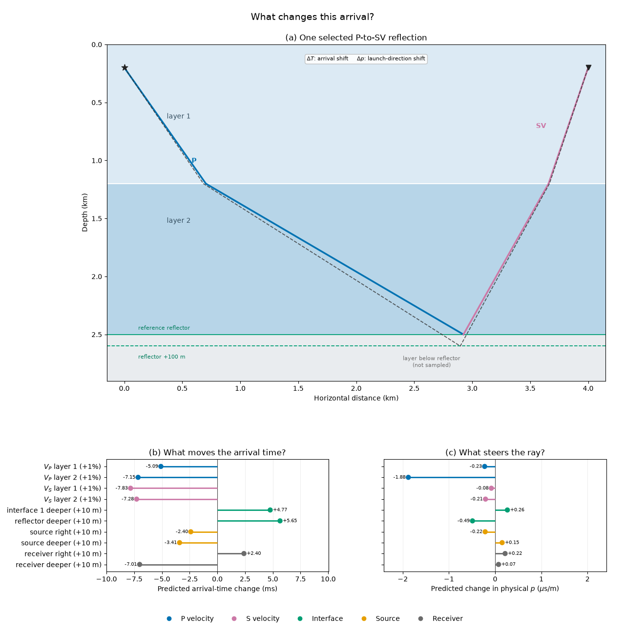
Sensitivity fingerprint for the labelled changes:
                    change  delta_time_ms  delta_parameter_us_per_m
       $V_P$ layer 1 (+1%)      -5.094302                 -0.227020
       $V_P$ layer 2 (+1%)      -7.148433                 -1.878979
       $V_S$ layer 1 (+1%)      -7.828732                 -0.082485
       $V_S$ layer 2 (+1%)      -7.281433                 -0.208807
interface 1 deeper (+10 m)       4.765143                  0.264952
  reflector deeper (+10 m)       5.651561                 -0.490669
      source right (+10 m)      -2.397292                 -0.215896
     source deeper (+10 m)      -3.407947                  0.151870
    receiver right (+10 m)       2.397292                  0.215896
   receiver deeper (+10 m)      -7.008757                  0.073846

How to read this figure. Panel (a) shows the selected ray in depth section. Blue is the downgoing P leg, magenta is the upgoing SV leg, and the black dashed path is the independently retraced ray after moving the reflector 100 m deeper. Only the two layers above the reflector are crossed, which explains why properties below it do not appear in the sensitivity fingerprint. The separation between the solid and dashed paths makes both consequences of a perturbation tangible: the arrival time changes and the takeoff direction changes.

Panel (b) converts every raw traveltime derivative into the effect of the labelled, physically small perturbation. A marker to the left of zero means an earlier arrival; a marker to the right means a later arrival. For example, increasing a sampled velocity shortens the traveltime, whereas deepening either crossed interface lengthens the path and delays the arrival. Equal and opposite horizontal source and receiver effects express the translational symmetry of the layered model.

Panel (c) applies the same perturbations to physical horizontal slowness \(p\). Changes in \(p\) alter takeoff direction and ray bending. Signs need not match those in panel (b): moving the reflector deeper delays this arrival, for example, but changes the launch direction in the opposite sense. The shared colors connect each parameter class across panels (b) and (c), while missing out-of-plane and below-reflector entries make the sparse derivative structure visible.

Use the derivatives as a local predictor

A model update usually changes several parameters at once. The predicted change is obtained by multiplying each perturbation by its derivative and adding the contributions. The random nearby models below are retraced only to verify that one reference sensitivity record predicts both outputs.

def perturb_and_predict(scale, random_generator):
    """Perturb all active parameter classes and compare with a retrace."""
    trial_model = model.copy()
    trial_source = source.copy()
    trial_receiver = receiver.copy()

    delta_vp = random_generator.normal(size=2) * 0.01 * scale * model.loc[[0, 1], "Vp"].to_numpy()
    delta_vs = random_generator.normal(size=2) * 0.01 * scale * model.loc[[0, 1], "Vs"].to_numpy()
    delta_interfaces = random_generator.normal(size=2) * 10.0 * scale
    delta_source = random_generator.normal(size=2) * 10.0 * scale
    delta_receiver = random_generator.normal(size=2) * 10.0 * scale

    trial_model.loc[[0, 1], "Vp"] += delta_vp
    trial_model.loc[[0, 1], "Vs"] += delta_vs
    trial_model.loc[[1, 2], "Depth"] += delta_interfaces
    trial_source[[0, 2]] += delta_source
    trial_receiver[[0, 2]] += delta_receiver

    delta_vp_full = np.zeros(len(model))
    delta_vs_full = np.zeros(len(model))
    delta_interfaces_full = np.zeros(len(model))
    delta_source_full = np.zeros(3)
    delta_receiver_full = np.zeros(3)
    delta_vp_full[[0, 1]] = delta_vp
    delta_vs_full[[0, 1]] = delta_vs
    delta_interfaces_full[[1, 2]] = delta_interfaces
    delta_source_full[[0, 2]] = delta_source
    delta_receiver_full[[0, 2]] = delta_receiver
    predicted = lt.linearized_ray_change(
        sensitivity,
        delta_vp=delta_vp_full,
        delta_vs=delta_vs_full,
        delta_interface_depths=delta_interfaces_full,
        delta_source=delta_source_full,
        delta_receiver=delta_receiver_full,
    )

    assert np.all(np.diff(trial_model["Depth"]) > 0.0)
    trial = trace_ps_reflection(
        trial_model,
        trial_source,
        trial_receiver,
        {"travel_times", "ray_parameters"},
    )
    exact_time = trial.travel_times[0] - reference.travel_times[0]
    exact_parameter = trial.ray_parameters[0] - reference.ray_parameters[0]
    return (
        predicted.delta_travel_time,
        exact_time,
        predicted.delta_ray_parameter,
        exact_parameter,
    )


scales = np.array([0.25, 1.0, 4.0])
comparisons = {}
relative_time_error = []
relative_parameter_error = []

for scale in scales:
    # Reuse the same perturbation directions at every scale so that this
    # comparison isolates the effect of moving farther from the reference.
    scale_rng = np.random.default_rng(7)
    values = np.array([perturb_and_predict(scale, scale_rng) for _ in range(80)])
    comparisons[scale] = values
    predicted_time, exact_time, predicted_parameter, exact_parameter = values.T
    relative_time_error.append(
        100.0 * np.sqrt(np.mean((predicted_time - exact_time) ** 2))
        / np.sqrt(np.mean(exact_time**2))
    )
    relative_parameter_error.append(
        100.0 * np.sqrt(np.mean((predicted_parameter - exact_parameter) ** 2))
        / np.sqrt(np.mean(exact_parameter**2))
    )

nominal_scale_index = int(np.flatnonzero(scales == 1.0)[0])
assert relative_time_error[nominal_scale_index] < 5.0
assert relative_parameter_error[nominal_scale_index] < 5.0

print("\nRelative RMS prediction error:")
for scale, time_error, parameter_error in zip(scales, relative_time_error, relative_parameter_error):
    print(f"  {scale:g}x: travel time {time_error:.2f}%, ray parameter {parameter_error:.2f}%")

nominal = comparisons[1.0]
predicted_time, exact_time, predicted_parameter, exact_parameter = nominal.T
figure, axes = plt.subplots(1, 3, figsize=(13.2, 4.4))


def prediction_panel(axis, exact, predicted, scale_factor, units, title):
    """Plot analytic predictions against independent retraces."""
    exact_scaled = scale_factor * exact
    predicted_scaled = scale_factor * predicted
    lower = min(exact_scaled.min(), predicted_scaled.min())
    upper = max(exact_scaled.max(), predicted_scaled.max())
    padding = 0.07 * (upper - lower)
    bounds = [lower - padding, upper + padding]
    axis.scatter(exact_scaled, predicted_scaled, s=24, color="#0072B2", alpha=0.65, edgecolors="none")
    axis.plot(bounds, bounds, color="#333333", linestyle="--", linewidth=1.0, label="perfect prediction")
    axis.set_xlim(bounds)
    axis.set_ylim(bounds)
    axis.set_aspect("equal", adjustable="box")
    axis.set_xlabel(f"Retraced change ({units})")
    axis.set_ylabel(f"Derivative prediction ({units})")
    axis.set_title(title)
    axis.legend(frameon=False, fontsize=8)
    axis.grid(alpha=0.2)


prediction_panel(
    axes[0],
    exact_time,
    predicted_time,
    1e3,
    "ms",
    "(a) Arrival-time changes",
)
prediction_panel(
    axes[1],
    exact_parameter,
    predicted_parameter,
    1e6,
    r"$\mu$s/m",
    r"(b) Physical $p$ changes",
)

axis = axes[2]
axis.plot(scales, relative_time_error, "o-", color="#0072B2", label="travel time")
axis.plot(scales, relative_parameter_error, "s-", color="#CC79A7", label="physical ray parameter")
axis.set_xscale("log", base=2)
axis.set_xticks(scales, [r"$\frac{1}{4}\times$", r"$1\times$", r"$4\times$"])
axis.set_xlabel("Perturbation size")
axis.set_ylabel("RMS prediction error\n(% of the exact change)")
axis.set_title("(c) Where is the local prediction useful?")
axis.legend(frameon=False, fontsize=8)
axis.grid(alpha=0.2)

active_derivatives = len(effects)
finite_difference_traces = 2 * active_derivatives + 1
figure.text(
    0.5,
    0.025,
    f"1 reference trace returns {active_derivatives} active parameter sensitivities; "
    f"a centered finite-difference Jacobian would require {finite_difference_traces} traces.",
    ha="center",
    va="bottom",
    fontsize=9.5,
    bbox={"boxstyle": "round,pad=0.4", "facecolor": "#F2F6F8", "edgecolor": "#AAB7BF"},
)
figure.suptitle("One traced ray predicts nearby rays", fontsize=14)
figure.subplots_adjust(left=0.07, right=0.985, top=0.84, bottom=0.25, wspace=0.34)
plt.show()

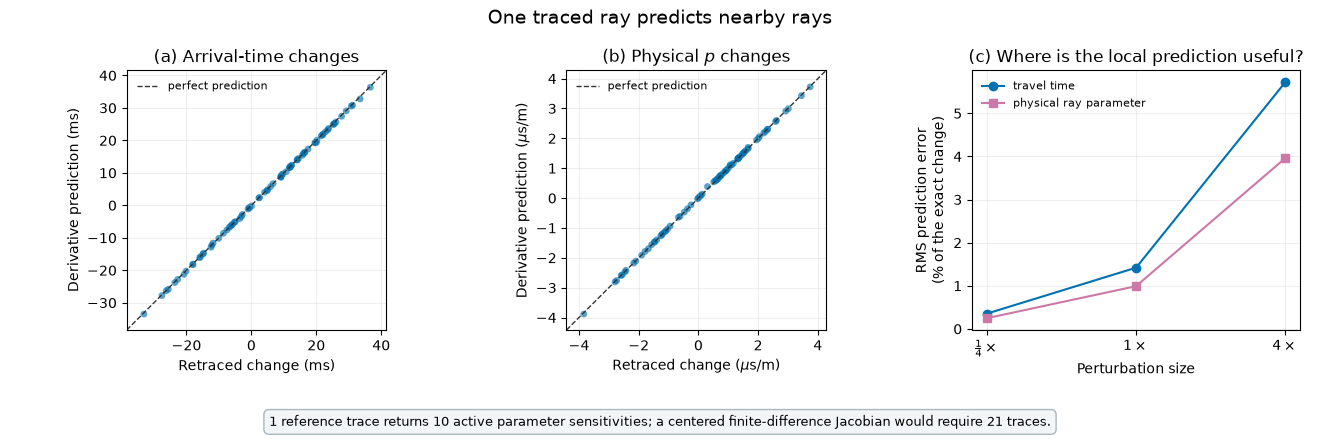
Relative RMS prediction error:
  0.25x: travel time 0.35%, ray parameter 0.25%
  1x: travel time 1.42%, ray parameter 0.99%
  4x: travel time 5.72%, ray parameter 3.96%

How to read this figure. Panels (a) and (b) compare the derivative prediction with a full retrace after simultaneously perturbing velocities, interfaces, and endpoint coordinates. Each dot is one deterministic nearby model. Dots on the dashed 1:1 line are exact first-order predictions; the tight alignment shows that one sensitivity record predicts both the traveltime change and the change in physical \(p\) without tracing a separate finite-difference ray for every parameter.

Panel (c) repeats the same perturbation directions at one quarter, nominal, and four times their original size. The error is normalized by the size of the actual response. Both curves grow smoothly with distance from the reference model, showing the expected local character of a linear approximation. The nominal perturbations remain close to the reference, while the four-times case begins to show where retracing or a new linearization point becomes useful. The annotation below the panels states the computational comparison: one analytic trace supplies 10 active sensitivities, whereas centered finite differences would require 21 traces.

# The analytic derivatives are local: the prediction is best for small changes
# that preserve the endpoint layers, selected P-to-SV itinerary, and
# propagating branch.  This first prediction experiment changes the model and
# acquisition geometry together; the next one isolates a practical
# traveltime-only use of the endpoint derivatives.

Predict travel times at nearby endpoints

Endpoint derivatives can replace many closely spaced ray solves with sparse exact anchor rays. For a nearby source and receiver, use the closest anchor pair and the first-order prediction

\[T \approx T_0 + \nabla_{\mathbf{s}}T\mathbin{\cdot}\Delta\mathbf{s} + \nabla_{\mathbf{r}}T\mathbin{\cdot}\Delta\mathbf{r}.\]

The example below contains 41 source positions and 161 receiver positions, or 6601 source–receiver pairs. The sources and receivers remain in the same layers, and every ray retains the selected P-to-SV reflection topology.

source_x = np.linspace(-200.0, 200.0, 41)
receiver_x = np.linspace(3600.0, 4400.0, 161)
dense_sources = np.column_stack([
    source_x,
    np.zeros_like(source_x),
    np.full_like(source_x, 200.0),
])
dense_receivers = np.column_stack([
    receiver_x,
    np.zeros_like(receiver_x),
    np.full_like(receiver_x, 200.0),
])

# Full retracing is performed only to measure the prediction error in this
# example.  A production approximation would calculate only the anchor rays.
dense_exact = trace_ps_reflection(
    model,
    dense_sources,
    dense_receivers,
    {"travel_times"},
)
exact_times = dense_exact.travel_times.reshape(len(dense_sources), len(dense_receivers))

dense_itinerary = lt.RayItinerary(
    source_phase="P",
    interactions=[lt.Interaction(float(model.iloc[2]["Depth"]), "reflect", "SV")],
)
anchor_distances = np.array([25.0, 50.0, 100.0])
approximators = {}
predictions = {}
anchor_counts = []
rms_errors_ms = []
maximum_errors_ms = []

for max_distance in anchor_distances:
    approximator = lt.TravelTimeApproximator.fit(
        dense_sources,
        dense_receivers,
        model,
        source_max_distance=max_distance,
        receiver_max_distance=max_distance,
        itinerary=dense_itinerary,
        n_jobs=1,
    )
    prediction = approximator.predict()
    assert prediction.valid_mask.all()
    predicted_times = prediction.travel_time_matrix
    error_ms = 1e3 * (predicted_times - exact_times)
    approximators[max_distance] = approximator
    predictions[max_distance] = predicted_times
    anchor_counts.append(approximator.exact_ray_count)
    rms_errors_ms.append(float(np.sqrt(np.mean(error_ms**2))))
    maximum_errors_ms.append(float(np.max(np.abs(error_ms))))

nominal_distance = 50.0
nominal_approximator = approximators[nominal_distance]
nominal_prediction = predictions[nominal_distance]
nominal_error_ms = 1e3 * (nominal_prediction - exact_times)
nominal_index = int(np.flatnonzero(anchor_distances == nominal_distance)[0])

assert rms_errors_ms[nominal_index] < 0.05
assert maximum_errors_ms[nominal_index] < 0.2

print("\nDense endpoint travel-time prediction:")
print(f"  Dense source-receiver pairs: {exact_times.size}")
for max_distance, count, rms_error, maximum_error in zip(
    anchor_distances, anchor_counts, rms_errors_ms, maximum_errors_ms
):
    print(
        f"  {max_distance:.0f} m maximum anchor distance: {count} exact rays, "
        f"RMS error {rms_error:.4f} ms, maximum error {maximum_error:.4f} ms"
    )

# Trace three representative rays only for the geometry panel.  The prediction
# itself still uses the 45 exact anchor pairs defined above.
middle_source_index = len(dense_sources) // 2
representative_receiver_indices = np.array([0, len(dense_receivers) // 2, len(dense_receivers) - 1])
representative = trace_ps_reflection(
    model,
    dense_sources[middle_source_index],
    dense_receivers[representative_receiver_indices],
    {"travel_times", "rays"},
)
nominal_source_anchor_indices = nominal_approximator.source_anchor_indices
nominal_receiver_anchor_indices = nominal_approximator.receiver_anchor_indices

Dense endpoint travel-time prediction:
  Dense source-receiver pairs: 6601
  25 m maximum anchor distance: 153 exact rays, RMS error 0.0070 ms, maximum error 0.0314 ms
  50 m maximum anchor distance: 45 exact rays, RMS error 0.0280 ms, maximum error 0.1275 ms
  100 m maximum anchor distance: 15 exact rays, RMS error 0.1127 ms, maximum error 0.5434 ms

Plot prediction accuracy

The nominal 50 m maximum endpoint-to-anchor distance uses sparse exact anchor rays to predict all 6601 travel times. The full dense result remains the validation reference, not an input to the prediction.

figure, axes = plt.subplots(2, 2, figsize=(12.8, 8.2))

axis = axes[0, 0]
axis.axhspan(0.0, 1.2, color="#DCEAF4")
axis.axhspan(1.2, 2.5, color="#B7D5E8")
axis.axhline(1.2, color="white", linewidth=1.4)
axis.axhline(2.5, color="#009E73", linewidth=1.3)
for ray_index, ray in enumerate(representative.rays):
    turning_index = int(np.argmax(ray[:, 2]))
    alpha = 1.0 if ray_index == 1 else 0.42
    linewidth = 2.2 if ray_index == 1 else 1.2
    axis.plot(
        ray[: turning_index + 1, 0] / 1000.0,
        ray[: turning_index + 1, 2] / 1000.0,
        color="#0072B2",
        linewidth=linewidth,
        alpha=alpha,
    )
    axis.plot(
        ray[turning_index:, 0] / 1000.0,
        ray[turning_index:, 2] / 1000.0,
        color="#CC79A7",
        linewidth=linewidth,
        alpha=alpha,
    )
axis.scatter(
    source_x / 1000.0,
    dense_sources[:, 2] / 1000.0,
    s=9,
    color=group_colors["Source"],
    label="41 sources (10 m spacing)",
    zorder=4,
)
axis.scatter(
    receiver_x / 1000.0,
    dense_receivers[:, 2] / 1000.0,
    s=7,
    color=group_colors["Receiver"],
    label="161 receivers (5 m spacing)",
    zorder=4,
)
axis.scatter(
    source_x[nominal_source_anchor_indices] / 1000.0,
    dense_sources[nominal_source_anchor_indices, 2] / 1000.0,
    s=42,
    facecolors="none",
    edgecolors="#A96700",
    linewidths=1.2,
    label=r"anchors ($\leq$50 m away)",
    zorder=5,
)
axis.scatter(
    receiver_x[nominal_receiver_anchor_indices] / 1000.0,
    dense_receivers[nominal_receiver_anchor_indices, 2] / 1000.0,
    s=42,
    facecolors="none",
    edgecolors="#333333",
    linewidths=1.2,
    zorder=5,
)
axis.text(0.0, 0.08, "source aperture", color="#A96700", ha="center", fontsize=8)
axis.text(4.0, 0.08, "receiver aperture", color="#444444", ha="center", fontsize=8)
axis.text(0.0, 2.45, "reflector at 2.5 km", color="#007C5B", va="bottom", fontsize=8)
axis.text(
    0.02,
    0.04,
    rf"{len(nominal_source_anchor_indices)} source anchors $\times$ "
    rf"{len(nominal_receiver_anchor_indices)} receiver anchors = "
    rf"{anchor_counts[nominal_index]} exact ray pairs",
    transform=axis.transAxes,
    fontsize=8,
    bbox={"boxstyle": "round,pad=0.3", "facecolor": "white", "alpha": 0.88, "edgecolor": "#BBBBBB"},
)
axis.set_xlim(-0.35, 4.55)
axis.set_ylim(2.7, 0.0)
axis.set_aspect("equal", adjustable="box")
axis.set_xlabel("Horizontal position (km)")
axis.set_ylabel("Depth (km)")
axis.set_title("(a) Source, receiver, and anchor geometry")
axis.legend(frameon=False, fontsize=7.5, loc="upper center", bbox_to_anchor=(0.52, 0.99))

axis = axes[0, 1]
exact_ms = 1e3 * exact_times.ravel()
predicted_ms = 1e3 * nominal_prediction.ravel()
bounds = [min(exact_ms.min(), predicted_ms.min()), max(exact_ms.max(), predicted_ms.max())]
axis.scatter(exact_ms, predicted_ms, s=8, color="#0072B2", alpha=0.22, edgecolors="none")
axis.plot(bounds, bounds, "--", color="#333333", linewidth=1.0, label="perfect prediction")
axis.set_xlim(bounds)
axis.set_ylim(bounds)
axis.set_aspect("equal", adjustable="box")
axis.set_xlabel("Fully retraced travel time (ms)")
axis.set_ylabel("Derivative prediction (ms)")
axis.set_title("(b) Dense travel-time matrix")
axis.legend(frameon=False, fontsize=8)
axis.grid(alpha=0.2)

axis = axes[1, 0]
image = axis.imshow(
    np.abs(nominal_error_ms),
    origin="lower",
    aspect="equal",
    extent=[receiver_x[0] / 1000.0, receiver_x[-1] / 1000.0, source_x[0] / 1000.0, source_x[-1] / 1000.0],
    cmap="magma",
)
axis.set_xlabel("Receiver position (km)")
axis.set_ylabel("Source position (km)")
axis.set_title("(c) Absolute error, 50 m maximum distance")
colorbar = figure.colorbar(image, ax=axis, pad=0.02)
colorbar.set_label("Absolute travel-time error (ms)")

axis = axes[1, 1]
axis.plot(anchor_distances, rms_errors_ms, "o-", color="#0072B2", label="RMS error")
axis.plot(anchor_distances, maximum_errors_ms, "s-", color="#D55E00", label="maximum error")
for max_distance, count, maximum_error in zip(anchor_distances, anchor_counts, maximum_errors_ms):
    axis.annotate(
        f"{count} anchors",
        (max_distance, maximum_error),
        xytext=(0, 8),
        textcoords="offset points",
        ha="center",
        fontsize=7.5,
    )
axis.set_xlabel("Maximum endpoint-to-anchor distance (m)")
axis.set_ylabel("Travel-time error (ms)")
axis.set_title("(d) Accuracy versus exact-ray count")
axis.legend(frameon=False, fontsize=8)
axis.grid(alpha=0.2)

figure.text(
    0.5,
    0.025,
    f"At 50 m maximum distance: {anchor_counts[nominal_index]} exact anchor rays predict "
    f"{exact_times.size} nearby travel times; RMS error = "
    f"{rms_errors_ms[nominal_index]:.3f} ms.",
    ha="center",
    va="bottom",
    fontsize=9.5,
    bbox={"boxstyle": "round,pad=0.4", "facecolor": "#F2F6F8", "edgecolor": "#AAB7BF"},
)
figure.suptitle("Predict dense travel times from sparse exact anchors", fontsize=14)
figure.subplots_adjust(left=0.08, right=0.965, top=0.91, bottom=0.12, hspace=0.38, wspace=0.28)
plt.show()

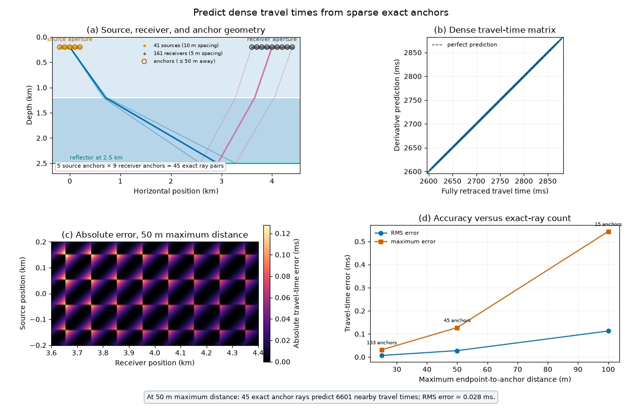
How to read this figure. Panel (a) defines the acquisition geometry for the endpoint-prediction experiment. All points lie in the same vertical plane at 200 m depth. The orange source aperture spans -0.2 to 0.2 km and contains 41 sources at 10 m spacing; the gray receiver aperture spans 3.6 to 4.4 km and contains 161 receivers at 5 m spacing. Open circles mark anchors selected automatically so that every endpoint lies within 50 m of one. Combining five source anchors with nine receiver anchors produces 45 exactly traced anchor rays. Three rays from the central source illustrate the common P-down/SV-up reflection at 2.5 km; all 6601 endpoint pairs use this topology.

Panel (b) compares every predicted traveltime with the independently retraced value. Each dot is one of the \(41\times161=6601\) source–receiver pairs. The dots collapse onto the dashed 1:1 line, so the prediction error is much smaller than the roughly 300 ms traveltime variation across the acquisition apertures. The full retraces are used only for validation in this example.

Panel (c) magnifies the small absolute errors for the 50 m maximum-distance model. The axes correspond directly to the receiver and source apertures in panel (a). Error is zero at an anchor and grows smoothly toward the midpoint between neighboring anchors, producing the repeated triangular pattern. Even the brightest locations remain below 0.13 ms.

Panel (d) exposes the accuracy–cost trade-off. A 25 m maximum distance uses 153 exact rays and gives the smallest errors. The nominal 50 m limit needs 45 rays and has 0.028 ms RMS error. With a 100 m limit only 15 exact rays are needed, but the maximum error rises to about 0.54 ms. Thus the plot provides a direct way to choose anchor distance for a desired traveltime tolerance.

These are local, fixed-topology predictions. Source and receiver layer membership, the P-to-SV itinerary, and the propagating branch must remain unchanged. Larger endpoint separations require closer anchors or full ray tracing; the error curve above makes that trade-off explicit.

Microseismic monitoring from a vertical receiver well

Consider a 1-km-deep monitoring well and a set of possible microseismic sources in a 2 km by 2 km region on one side of it. Ten receivers are fixed in the well. Direct P-wave traveltimes are needed from every possible source location to every receiver, for example when scanning a location grid.

The dense calculation below traces all 1640 source locations to all 10 receivers. The anchored calculation traces every receiver only from a coarser subset of source locations. Traveltimes at neighboring source points are predicted with the analytic source-coordinate derivatives and fixed-topology endpoint curvature (order=2). LayTracer places initial point-cloud anchors within each layer and refines them until every source–receiver pair has a nearby anchor with the same ordered layer, phase, and vertical-direction topology.

micro_model = pd.DataFrame({
    "Depth": [0.0, 700.0, 1400.0],
    "Vp": [2600.0, 3400.0, 4300.0],
    "Vs": [1450.0, 1950.0, 2500.0],
})
micro_source_x = np.arange(0.0, 2000.0 + 50.0, 50.0)
micro_source_z = np.arange(25.0, 2000.0, 50.0)
micro_grid_x, micro_grid_z = np.meshgrid(micro_source_x, micro_source_z)
micro_sources = np.column_stack([
    micro_grid_x.ravel(),
    np.zeros(micro_grid_x.size),
    micro_grid_z.ravel(),
])
micro_receivers = np.column_stack([
    np.zeros(10),
    np.zeros(10),
    np.arange(100.0, 1000.0 + 100.0, 100.0),
])


def trace_direct_p(sources_to_trace, receivers_to_trace, requested):
    """Trace direct P arrivals for the microseismic experiment."""
    return lt.trace_rays(
        sources_to_trace,
        receivers_to_trace,
        micro_model,
        source_phase="P",
        requested=requested,
        n_jobs=1,
        verbose=False,
        tol=1e-10,
        max_iter=30,
    )


start = time.perf_counter()
micro_exact = trace_direct_p(micro_sources, micro_receivers, {"travel_times"})
micro_full_trace_seconds = time.perf_counter() - start
micro_exact_times = micro_exact.travel_times.reshape(len(micro_sources), len(micro_receivers))
micro_anchor_distances = np.array([75.0, 150.0, 300.0])
micro_approximators = {}
micro_predictions = {}
micro_anchor_sources = {}
micro_exact_ray_counts = []
micro_rms_errors_ms = []
micro_maximum_errors_ms = []
micro_anchor_setup_seconds = []
micro_prediction_seconds = []
micro_approximation_seconds = []

for max_distance in micro_anchor_distances:
    start = time.perf_counter()
    approximator = lt.TravelTimeApproximator.fit(
        micro_sources,
        micro_receivers,
        micro_model,
        source_max_distance=max_distance,
        receiver_max_distance=None,
        source_phase="P",
        n_jobs=1,
        tol=1e-10,
        max_iter=30,
    )
    micro_anchor_setup_seconds.append(time.perf_counter() - start)
    start = time.perf_counter()
    prediction = approximator.predict(order=2)
    micro_prediction_seconds.append(time.perf_counter() - start)
    micro_approximation_seconds.append(
        micro_anchor_setup_seconds[-1] + micro_prediction_seconds[-1]
    )
    assert prediction.valid_mask.all()
    predicted_times = prediction.travel_time_matrix
    error_ms = 1e3 * (predicted_times - micro_exact_times)
    micro_approximators[max_distance] = approximator
    micro_predictions[max_distance] = predicted_times
    micro_anchor_sources[max_distance] = approximator.anchor_sources
    micro_exact_ray_counts.append(approximator.exact_ray_count)
    micro_rms_errors_ms.append(float(np.sqrt(np.mean(error_ms**2))))
    micro_maximum_errors_ms.append(float(np.max(np.abs(error_ms))))

micro_nominal_distance = 150.0
micro_nominal_index = int(
    np.flatnonzero(micro_anchor_distances == micro_nominal_distance)[0]
)
micro_nominal_prediction = micro_predictions[micro_nominal_distance]
micro_nominal_error_ms = 1e3 * (micro_nominal_prediction - micro_exact_times)
micro_nominal_absolute_error_ms = np.abs(micro_nominal_error_ms)
micro_percentile_95_ms = float(np.percentile(micro_nominal_absolute_error_ms, 95.0))
micro_source_rms_error_ms = np.sqrt(np.mean(micro_nominal_error_ms**2, axis=1)).reshape(
    micro_grid_x.shape
)

assert micro_exact_times.size == 16400
assert micro_exact_ray_counts[micro_nominal_index] < micro_exact_times.size

print("\nMicroseismic source-grid traveltime prediction:")
print(
    f"  Full calculation: {micro_exact_times.size} exact rays in "
    f"{micro_full_trace_seconds:.3f} s (single process)"
)
print("  Anchor setup and prediction are timed separately (machine-dependent):")
for (
    max_distance,
    ray_count,
    rms_error,
    maximum_error,
    setup_seconds,
    prediction_seconds,
    approximation_seconds,
) in zip(
    micro_anchor_distances,
    micro_exact_ray_counts,
    micro_rms_errors_ms,
    micro_maximum_errors_ms,
    micro_anchor_setup_seconds,
    micro_prediction_seconds,
    micro_approximation_seconds,
):
    speedup = micro_full_trace_seconds / approximation_seconds
    print(
        f"  {max_distance:.0f} m maximum source-anchor distance: {ray_count} exact rays, "
        f"setup {setup_seconds:.3f} s + prediction {prediction_seconds:.3f} s = "
        f"{approximation_seconds:.3f} s ({speedup:.2f}x versus full trace), "
        f"RMS error {rms_error:.4f} ms, maximum error {maximum_error:.4f} ms"
    )
print(
    f"  150 m maximum distance: 95% of absolute errors below "
    f"{micro_percentile_95_ms:.4f} ms"
)

assert micro_rms_errors_ms[micro_nominal_index] < 5.0

Microseismic source-grid traveltime prediction:
  Full calculation: 16400 exact rays in 1.997 s (single process)
  Anchor setup and prediction are timed separately (machine-dependent):
  75 m maximum source-anchor distance: 3470 exact rays, setup 1.125 s + prediction 0.726 s = 1.851 s (1.08x versus full trace), RMS error 0.0515 ms, maximum error 5.4750 ms
  150 m maximum source-anchor distance: 1660 exact rays, setup 0.710 s + prediction 0.672 s = 1.382 s (1.44x versus full trace), RMS error 0.1143 ms, maximum error 5.4750 ms
  300 m maximum source-anchor distance: 630 exact rays, setup 0.276 s + prediction 0.643 s = 0.919 s (2.17x versus full trace), RMS error 0.9384 ms, maximum error 49.2564 ms
  150 m maximum distance: 95% of absolute errors below 0.0895 ms

Plot the monitoring geometry and prediction errors

The nominal comparison limits every source to a topology-compatible anchor no farther than 150 m away. The full dense solution is validation only.

micro_geometry_sources = np.array([
    [250.0, 0.0, 325.0],
    [900.0, 0.0, 775.0],
    [1500.0, 0.0, 1275.0],
    [1950.0, 0.0, 1875.0],
])
micro_geometry_receiver = micro_receivers[5]
micro_geometry_rays = trace_direct_p(
    micro_geometry_sources,
    micro_geometry_receiver,
    {"travel_times", "rays"},
)

figure, axes = plt.subplots(2, 2, figsize=(12.8, 8.4))

axis = axes[0, 0]
axis.fill_betweenx([0.0, 0.7], 0.0, 2.0, color="#DCEAF4")
axis.fill_betweenx([0.7, 1.4], 0.0, 2.0, color="#B7D5E8")
axis.fill_betweenx([1.4, 2.05], 0.0, 2.0, color="#95C0DA")
axis.hlines([0.7, 1.4], 0.0, 2.0, color="white", linewidth=1.3)
axis.scatter(
    micro_sources[:, 0] / 1000.0,
    micro_sources[:, 2] / 1000.0,
    s=4,
    color="#5F7482",
    alpha=0.28,
    label="1640 possible sources",
)
nominal_micro_anchors = micro_anchor_sources[micro_nominal_distance]
axis.scatter(
    nominal_micro_anchors[:, 0] / 1000.0,
    nominal_micro_anchors[:, 2] / 1000.0,
    s=19,
    facecolors="none",
    edgecolors="#D55E00",
    linewidths=0.8,
    label=f"{len(nominal_micro_anchors)} source anchors",
    zorder=3,
)
axis.plot([0.0, 0.0], [0.0, 1.0], color="#222222", linewidth=1.8, label="1 km well")
axis.scatter(
    micro_receivers[:, 0] / 1000.0,
    micro_receivers[:, 2] / 1000.0,
    marker=">",
    s=35,
    color="#222222",
    label="10 receivers",
    zorder=5,
)
for ray in micro_geometry_rays.rays:
    axis.plot(
        ray[:, 0] / 1000.0,
        ray[:, 2] / 1000.0,
        color="#0072B2",
        linewidth=1.4,
        alpha=0.75,
    )
axis.text(1.77, 0.38, r"$V_P=2.6$ km/s", color="#354F60", fontsize=8)
axis.text(1.77, 1.08, r"$V_P=3.4$ km/s", color="#354F60", fontsize=8)
axis.text(1.77, 1.76, r"$V_P=4.3$ km/s", color="#354F60", fontsize=8)
axis.set_xlim(-0.12, 2.08)
axis.set_ylim(2.05, 0.0)
axis.set_aspect("equal", adjustable="box")
axis.set_xlabel("Distance from monitoring well (km)")
axis.set_ylabel("Depth (km)")
axis.set_title("(a) Vertical-well monitoring geometry")
axis.legend(
    frameon=False,
    fontsize=7.3,
    loc="upper left",
    bbox_to_anchor=(1.02, 0.98),
    borderaxespad=0.0,
)

axis = axes[0, 1]
micro_exact_ms = 1e3 * micro_exact_times.ravel()
micro_predicted_ms = 1e3 * micro_nominal_prediction.ravel()
micro_bounds = [
    min(micro_exact_ms.min(), micro_predicted_ms.min()),
    max(micro_exact_ms.max(), micro_predicted_ms.max()),
]
axis.scatter(
    micro_exact_ms,
    micro_predicted_ms,
    s=7,
    color="#0072B2",
    alpha=0.20,
    edgecolors="none",
)
axis.plot(micro_bounds, micro_bounds, "--", color="#333333", linewidth=1.0, label="perfect prediction")
axis.set_xlim(micro_bounds)
axis.set_ylim(micro_bounds)
axis.set_aspect("equal", adjustable="box")
axis.set_xlabel("Fully traced traveltime (ms)")
axis.set_ylabel("Second-order anchor prediction (ms)")
axis.set_title("(b) All 16,400 source--receiver times")
axis.legend(frameon=False, fontsize=8)
axis.grid(alpha=0.2)

axis = axes[1, 0]
image = axis.pcolormesh(
    micro_source_x / 1000.0,
    micro_source_z / 1000.0,
    micro_source_rms_error_ms,
    shading="nearest",
    cmap="magma",
)
axis.axhline(0.7, color="white", linewidth=0.8, alpha=0.8)
axis.axhline(1.4, color="white", linewidth=0.8, alpha=0.8)
axis.plot([0.0, 0.0], [0.0, 1.0], color="#00B8D9", linewidth=2.2)
axis.scatter(
    micro_receivers[:, 0] / 1000.0,
    micro_receivers[:, 2] / 1000.0,
    marker=">",
    s=24,
    color="#00B8D9",
    zorder=4,
)
axis.set_xlim(0.0, 2.0)
axis.set_ylim(2.0, 0.0)
axis.set_aspect("equal", adjustable="box")
axis.set_xlabel("Distance from monitoring well (km)")
axis.set_ylabel("Potential source depth (km)")
axis.set_title("(c) RMS error over the 10 receivers")
colorbar = figure.colorbar(image, ax=axis, pad=0.02)
colorbar.set_label("RMS traveltime error (ms)")

axis = axes[1, 1]
axis.plot(
    micro_anchor_distances,
    micro_rms_errors_ms,
    "o-",
    color="#0072B2",
    label="RMS error",
)
axis.plot(
    micro_anchor_distances,
    micro_maximum_errors_ms,
    "s-",
    color="#D55E00",
    label="maximum error",
)
for max_distance, ray_count, maximum_error in zip(
    micro_anchor_distances,
    micro_exact_ray_counts,
    micro_maximum_errors_ms,
):
    axis.annotate(
        f"{ray_count} rays",
        (max_distance, maximum_error),
        xytext=(0, 7),
        textcoords="offset points",
        ha="center",
        fontsize=7.5,
    )
axis.axhline(1.0, color="#666666", linestyle=":", linewidth=1.0, label="1 ms")
axis.set_yscale("log")
axis.set_xlabel("Maximum source-to-anchor distance (m)")
axis.set_ylabel("Traveltime error (ms, log scale)")
axis.set_title("(d) Accuracy versus exact-ray count")
axis.legend(frameon=False, fontsize=8)
axis.grid(alpha=0.2, which="both")
axis.margins(x=0.08, y=0.16)

micro_reduction = micro_exact_times.size / micro_exact_ray_counts[micro_nominal_index]
figure.text(
    0.5,
    0.022,
    f"At 150 m maximum distance: {micro_exact_ray_counts[micro_nominal_index]} exact rays "
    f"predict {micro_exact_times.size} traveltimes ({micro_reduction:.1f}$\\times$ fewer solves); "
    f"RMS error = {micro_rms_errors_ms[micro_nominal_index]:.2f} ms.",
    ha="center",
    va="bottom",
    fontsize=9.5,
    bbox={"boxstyle": "round,pad=0.4", "facecolor": "#F2F6F8", "edgecolor": "#AAB7BF"},
)
figure.suptitle("Approximate a microseismic traveltime table from source anchors", fontsize=14)
figure.subplots_adjust(left=0.08, right=0.965, top=0.91, bottom=0.11, hspace=0.36, wspace=0.28)
plt.show()

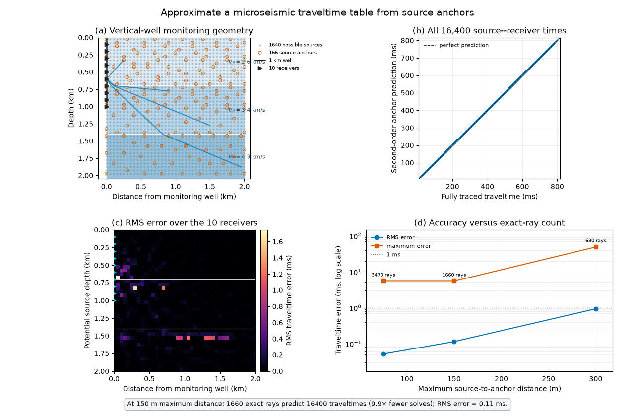
How to read this figure. Panel (a) shows the complete monitoring setup in depth section. The black vertical line is the 1-km well and the triangles are its 10 receivers. Small gray points are the 1640 possible event locations covering the one-sided 0–2 km horizontal and depth search region. Orange circles are the 166 source anchors selected for the nominal 150 m maximum distance. Blue examples illustrate direct P rays through the three velocity layers; refraction at 0.7 and 1.4 km is visible as a change in ray slope.

Panel (b) contains all 16,400 source–receiver traveltimes. The horizontal coordinate is obtained by fully tracing every ray, while the vertical coordinate is predicted to second order from the nearest topology-compatible source anchor. The point cloud follows the dashed 1:1 line over the full traveltime range. The small deviations cannot be judged reliably at this scale, so panels (c) and (d) display them directly.

Panel (c) maps the RMS prediction error at every possible source location, averaged over the 10 receivers. The well and receivers are repeated in cyan to connect the error pattern to the acquisition geometry. Errors are lowest at and near anchors and generally increase between their coverage regions. The second-order correction removes most of the horizontal bands around receiver depths that appear with a linear predictor. The remaining largest local errors occur where a short source–receiver path approaches an interface, so curvature is strong while the fixed-topology constraint prevents crossing that interface. Layer-aware and receiver-side-aware anchor selection prevents predictions from reversing the local ray branch; the white lines mark the two model interfaces.

Panel (d) summarizes the accuracy–cost trade-off on a logarithmic error scale. A 75 m distance limit uses 3470 exact rays and gives 0.052 ms RMS error. The nominal 150 m limit uses 1660 rays instead of 16,400—9.9 times fewer solves—with 0.114 ms RMS error, and 95% of individual absolute errors are below 0.090 ms. At 300 m only 630 rays are traced, but the RMS error rises to 0.94 ms. Maximum errors are much larger than RMS errors because a small number of short paths lie close to an interface; such regions are natural candidates for denser anchors or direct tracing.

This experiment treats the fully traced table as validation only. In a location scan, the anchored table would be the computational product: exact rays are calculated at the anchors and neighboring traveltimes are filled in analytically, with maximum anchor distance chosen from the acceptable error.