02. Paper examples

Reproducing three characteristic figures from paper:

Fang, X., & Chen, X. (2019). A fast and robust two-point ray tracing method in layered media with constant or linearly varying layer velocity. Geophysical Prospecting, 67(7), 1811–1824. https://doi.org/10.1111/1365-2478.12799 [Fang and Chen, 2019].

Setup

import laytracer as lt
import numpy as np
import pandas as pd
import matplotlib.pyplot as plt

# sphinx_gallery_thumbnail_number = -1

Reproduce Figure 9

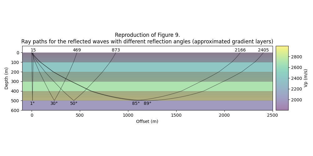
Here we reproduce Figure 9 from Fang and Chen [2019].

Figure 9 illustrates the ray paths for reflected waves in a five-layered model with mixed constant and gradient velocity layers. The model consists of:

• Layer 1 (0-100m): Gradient velocity \(v = 4z + 1800\)

• Layer 2 (100-200m): Constant velocity \(v = 2400\)

• Layer 3 (200-300m): Gradient velocity \(v = z + 2400\)

• Layer 4 (300-400m): Constant velocity \(v = 2700\)

• Layer 5 (400-500m): Gradient velocity \(v = 1.5z + 2250\)

The figure demonstrates the method’s capability to handle complex models with both constant and gradient layers. It shows rays with reflection angles of 1°, 30°, 50°, and (in the paper) 89° at the bottom interface (500m depth).

print("Reproducing Figure 9...")

layers = []
# Layer 1 (Gradient)
layers.append(lt.model.discretize_gradient_layer(0, 100, lambda z: 4*z + 1800))
# Layer 2 (Constant)
layers.append(pd.DataFrame({"Depth": [100.0], "Vp": [2400.0], "Vs": [2400.0/1.732], "Rho": [2500.0]}))
# Layer 3 (Gradient)
layers.append(lt.model.discretize_gradient_layer(200, 300, lambda z: z + 2400))
# Layer 4 (Constant)
layers.append(pd.DataFrame({"Depth": [300.0], "Vp": [2700.0], "Vs": [2700.0/1.732], "Rho": [2500.0]}))
# Layer 5 (Gradient) - We need this to go down to 500m
layers.append(lt.model.discretize_gradient_layer(400, 500, lambda z: 1.5*z + 2250))

# Add dummy half-space at 500m so it's a valid interface
layers.append(pd.DataFrame({"Depth": [500.0], "Vp": [2000.0], "Vs": [2000.0/1.732], "Rho": [2500.0]}))

vel_df = pd.concat(layers, ignore_index=True)

src = np.array([0.0, 0.0, 0.0])

# Target reflection angles at bottom (500m)
# Reduced set to avoid numerical instability with grazing rays in discretized model
angles_deg = np.array([1, 30, 50, 85, 89])

v_ref = 3000.0
p_targets = np.sin(np.deg2rad(angles_deg)) / v_ref

# Calculate target offsets
stack = lt.build_layer_stack(vel_df, 0.0, 500.0)
h = stack.h
v = stack.vp
vmax = np.max(v)
lmd = v / vmax
q_vals = lt.solver.q_from_p(p_targets, vmax)

offsets_half = []
for q in q_vals:
    x = lt.solver.offset(q, h, lmd)
    offsets_half.append(x)

offsets_total = np.array(offsets_half) * 2.0

receivers = np.zeros((len(offsets_total), 3))
receivers[:, 0] = offsets_total

print(f"Tracing rays for {len(receivers)} receivers...")
try:
    results = lt.trace_rays(
        sources=src,
        receivers=receivers,
        velocity_df=vel_df,
        source_phase="P",
        reflection=[(500.0, "P")]
    )
    print("Figure 9 Tracing complete.")
except Exception as e:
    print(f"Error tracing rays in Fig 9: {e}")
    raise e

fig, ax = plt.subplots(figsize=(10, 5))
lt.plot.rays_2d(
    vel_df=vel_df,
    rays=results.rays,
    vel_type="Vp",
    ax=ax,
    xlim=(-100, 2500),
    ylim=(600, -70),
    plot_model=True,
    add_colorbar=True,
    model_alpha=0.5
)
for i, x in enumerate(offsets_total):
    ax.text(x, 0, f"{offsets_total[i]:.0f}", ha='center', va='bottom')
    ax.text(x/2, 510, f"{angles_deg[i]}°", ha='center', va='top')

ax.set_title("Reproduction of Figure 9.\nRay paths for the reflected waves with different reflection angles (approximated gradient layers)")
ax.set_xlabel("Offset (m)")
ax.set_ylabel("Depth (m)")
fig.tight_layout()
plt.show()

Reproducing Figure 9...
Tracing rays for 5 receivers...
Figure 9 Tracing complete.

Reproduce Figure 10

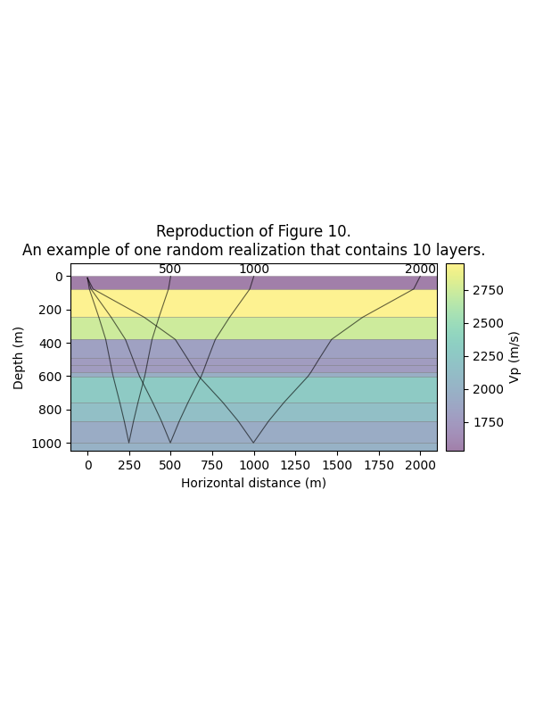
Here we reproduce Figure 10 from Fang and Chen [2019].

Figure 10 presents a random realization of a 10-layered model used for Monte Carlo simulations to test robustness. In the paper’s experimental setup:

• The model contains 10 layers with random thicknesses (uniform distribution corresponding to ~18-189 m).

• Layer velocities vary randomly between 1500 and 3000 m/s.

• The source is located at 10 m depth.

• Rays are traced to receivers at offsets of 500, 1000, and 2000 m.

This setup tests the q-method’s stability against random velocity fluctuations and layer thickness variations.

print("Reproducing Figure 10...")
np.random.seed(42)
n_layers = 10
total_depth = 1000.0
h_raw = np.random.uniform(18, 189, n_layers)
h_vals = h_raw * (total_depth / np.sum(h_raw))

depths_top = np.concatenate(([0], np.cumsum(h_vals[:-1])))
v_vals = np.random.uniform(1500, 3000, n_layers)

df_data = {
    "Depth": depths_top,
    "Vp": v_vals,
    "Vs": v_vals / 1.732,
    "Rho": 2500.0
}
vel_df = pd.DataFrame(df_data)

# Add dummy half-space
dummy_row = pd.DataFrame({
    "Depth": [1000.0],
    "Vp": [2000.0],
    "Vs": [2000.0/1.732],
    "Rho": [2500.0]
})
vel_df = pd.concat([vel_df, dummy_row], ignore_index=True)

src = np.array([0.0, 0.0, 10.0])
targets = np.array([500.0, 1000.0, 2000.0])
receivers = np.zeros((len(targets), 3))
receivers[:, 0] = targets

try:
    results = lt.trace_rays(
        sources=src,
        receivers=receivers,
        velocity_df=vel_df,
        source_phase="P",
        reflection=[(1000.0, "P")]
    )
    print("Figure 10 Tracing complete.")
except Exception as e:
    print(f"Error tracing rays in Fig 10: {e}")
    raise e

fig, ax = plt.subplots(figsize=(6, 8))
lt.plot.rays_2d(
    vel_df=vel_df,
    rays=results.rays,
    vel_type="Vp",
    ax=ax,
    ylim=(1050, -80),
    plot_model=True,
    add_colorbar=True,
    model_alpha=0.5
)
for i, x in enumerate(targets):
    ax.text(x, 0, f"{targets[i]:.0f}", ha='center', va='bottom')

ax.set_title("Reproduction of Figure 10.\nAn example of one random realization that contains 10 layers.")
fig.tight_layout()
plt.show()

Reproducing Figure 10...
Figure 10 Tracing complete.

Reproduce Figure 15c

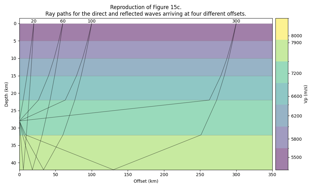
Here we reproduce Figure 15c from Fang and Chen [2019].

Figure 15c compares the q-method with the method of Kim and Baag (2002) using “Model I” from their paper. This serves as a crustal model benchmark with six constant-velocity layers:

• Layer 1 (0-5 km): 5.5 km/s

• Layer 2 (5-10 km): 5.8 km/s

• Layer 3 (10-15 km): 6.2 km/s

• Layer 4 (15-22 km): 6.6 km/s

• Layer 5 (22-32 km): 7.2 km/s

• Layer 6 (32-42 km): 7.9 km/s

• Layer 7 (>42 km): 8.0 km/s

The figure displays ray paths for both direct and reflected waves arriving at offsets of 20, 60, 100, and 300 km.

print("Reproducing Figure 15c...")
depths = np.array([0.0, 5.0, 10.0, 15.0, 22.0, 32.0, 42.0]) * 1000.0
vp = np.array([5.5, 5.8, 6.2, 6.6, 7.2, 7.9, 8.0]) * 1000.0

vel_df = pd.DataFrame({
    "Depth": depths,
    "Vp": vp,
    "Vs": vp / 1.732,
    "Rho": 2500.0
})

offsets_km = np.array([20, 60, 100, 300])
offsets_m = offsets_km * 1000.0
src = np.array([0.0, 0.0, 28000.0])
receivers = np.zeros((len(offsets_m), 3))
receivers[:, 0] = offsets_m

try:
    res_refl = lt.trace_rays(
        sources=src,
        receivers=receivers,
        velocity_df=vel_df,
        source_phase="P",
        reflection=[(42000.0, "P")]
    )
    res_refr = lt.trace_rays(
        sources=src,
        receivers=receivers,
        velocity_df=vel_df,
        source_phase="P"
    )

    print("Figure 15c Tracing complete.")
except Exception as e:
    print(f"Error tracing rays in Fig 15c: {e}")
    raise e

# Concatenate rays from both results
res_rays = res_refl.rays + res_refr.rays

fig, ax = plt.subplots(figsize=(10, 6))
lt.plot.rays_2d(
    vel_df=vel_df,
    rays=res_rays,
    vel_type="Vp",
    ax=ax,
    xlim=(0, 350),
    ylim=(42, -1.5),
    plot_model=True,
    equal_scale=False,
    add_colorbar=True,
    discrete_colorbar=True,
    model_alpha=0.5,
    unit="km"
)
for i, x in enumerate(offsets_km):
    ax.text(x, 0, f"{offsets_km[i]:.0f}", ha='center', va='bottom')

ax.set_title("Reproduction of Figure 15c.\nRay paths for the direct and reflected waves arriving at four different offsets.")
ax.set_xlabel("Offset (km)")
ax.set_ylabel("Depth (km)")
fig.tight_layout()
plt.show()

Reproducing Figure 15c...
Figure 15c Tracing complete.

References

[1] (1,2,3,4)

X. Fang and X. Chen. A fast and robust two‐point ray tracing method in layered media with constant or linearly varying layer velocity. Geophysical Prospecting, 67(7):1648–1661, 2019. doi:10.1111/1365-2478.12799.