Note
Go to the end to download the full example code.
05. Homogeneous equivalence quality check#
A two-layer model whose layers share identical elastic parameters must reproduce the closed-form homogeneous-medium solution exactly. This example computes travel time, \(t^*\), geometrical spreading, the transmission- coefficient product, and their combined deterministic factor for three cases:
where \(T = \prod |T_k|\) is the transmission-coefficient product and \(L\) is the relative geometrical spreading.
Interpretation of each factor:
\(t^*\) captures attenuation effects (intrinsic and scattering) along the ray path.
\(T\) captures interface effects (energy partition at each crossing). If an interface is physically invisible (identical elastic parameters above and below), its transmission magnitude is 1, so it should not alter amplitudes.
\(L\) captures ray-tube divergence/convergence (pure geometry and kinematics) through the relative geometrical spreading factor.
\(C = T/L\) is therefore the deterministic, frequency-independent part of amplitude scaling.
Including attenuation, a common form is
so this example checks separately that both attenuation (\(t^*\)) and deterministic scaling (\(T/L\)) remain unchanged when replacing a true homogeneous medium with an equivalent two-layer representation.
The expected physics for this benchmark is strict equivalence:
identical travel times and ray parameters,
identical \(t^*\), spreading, \(T\), and \(T/L\),
overlapping ray geometries and offset-dependent curves,
only machine-precision numerical differences.
It is therefore a powerful quality check for the internal consistency of the code, and a regression test to catch any future changes that might break this fundamental equivalence. The three approaches to compute the same physical quantities are:
Analytical formulas for a homogeneous medium.
LayTracer with a single-layer (homogeneous) model.
(c) LayTracer with a two-layer model where both layers have the same Vp, Vs, ρ, Qp, Qs.
All three must agree, confirming internal consistency of the code.
Setup#
import laytracer as lt
import numpy as np
import pandas as pd
import matplotlib.pyplot as plt

# sphinx_gallery_thumbnail_number = 2
Common parameters#
We use a single set of elastic constants and a fixed source-receiver geometry throughout the example.
VP = 5000.0       # P-wave velocity  (m/s)
VS = VP / 1.732   # S-wave velocity  (m/s)
RHO = 2700.0      # density          (kg/m³)
QP = 500.0        # P-wave quality factor
QS = 250.0        # S-wave quality factor

src = np.array([0.0, 0.0, 500.0])       # source at 500 m depth
rcv = np.array([5000.0, 0.0, 2500.0])   # receiver at 2500 m depth

epic = np.sqrt((rcv[0] - src[0]) ** 2 + (rcv[1] - src[1]) ** 2)
dz = abs(rcv[2] - src[2])
dist = np.sqrt(epic ** 2 + dz ** 2)

print(f"Epicentral distance: {epic:.1f} m")
print(f"Depth offset:        {dz:.1f} m")
print(f"Straight-ray length: {dist:.4f} m")
Epicentral distance: 5000.0 m
Depth offset:        2000.0 m
Straight-ray length: 5385.1648 m
(a) Analytical homogeneous solution#
In a homogeneous medium a ray is a straight line of length \(R = \sqrt{X^2 + \Delta z^2}\), giving:
tt_a  = dist / VP
p_a   = epic / (VP * dist)
ts_a  = tt_a / QP
L_a   = dist * VP
T_a   = 1.0
C_a   = T_a / L_a                # combined deterministic amplitude factor

print(f"\n--- Analytical ---")
print(f"Travel time:      {tt_a:.8f} s")
print(f"Ray parameter:    {p_a:.10e} s/m")
print(f"t*:               {ts_a:.10e} s")
print(f"Spreading:        {L_a:.4f}")
print(f"Trans. product:   {T_a:.6f}")
print(f"Combined (T/L):   {C_a:.10e}")
--- Analytical ---
Travel time:      1.07703296 s
Ray parameter:    1.8569533818e-04 s/m
t*:               2.1540659229e-03 s
Spreading:        26925824.0357
Trans. product:   1.000000
Combined (T/L):   3.7139067635e-08
(b) Homogeneous model via LayTracer#
A single-layer DataFrame - the simplest possible model.
homo_df = pd.DataFrame({
    "Depth": [0.0],
    "Vp":    [VP],
    "Vs":    [VS],
    "Rho":   [RHO],
    "Qp":    [QP],
    "Qs":    [QS],
})

res_h = lt.trace_rays(
    sources=src,
    receivers=rcv,
    velocity_df=homo_df,
    source_phase="P",
    requested={"travel_times", "rays", "ray_parameters", "tstar", "spreading", "trans_product"},
    transcoef_method="standard",
)

tt_h  = float(res_h.travel_times[0])
p_h   = float(res_h.ray_parameters[0])
ts_h  = float(res_h.tstar[0])
L_h   = float(res_h.spreading[0])
T_h   = float(res_h.trans_product[0])
C_h   = T_h / L_h

print(f"\n--- Homogeneous code ---")
print(f"Travel time:      {tt_h:.8f} s")
print(f"Ray parameter:    {p_h:.10e} s/m")
print(f"t*:               {ts_h:.10e} s")
print(f"Spreading:        {L_h:.4f}")
print(f"Trans. product:   {T_h:.6f}")
print(f"Combined (T/L):   {C_h:.10e}")
--- Homogeneous code ---
Travel time:      1.07703296 s
Ray parameter:    1.8569533818e-04 s/m
t*:               2.1540659229e-03 s
Spreading:        26925824.0357
Trans. product:   1.000000
Combined (T/L):   3.7139067635e-08
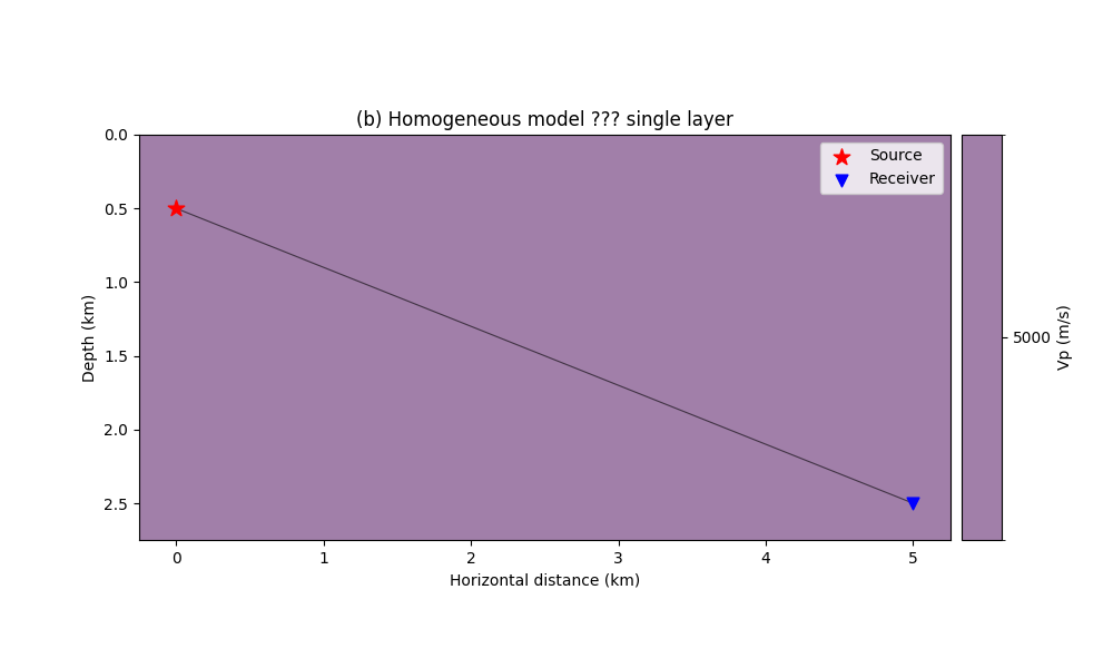
Plot the ray through the homogeneous model#
ax = lt.plot.rays_2d(
    homo_df,
    rays=res_h.rays,
    sources=np.atleast_2d(src),
    receivers=np.atleast_2d(rcv),
    vel_type="Vp",
    add_colorbar=True,
    model_alpha=0.5,
    discrete_colorbar=True,
    unit="km",
)
ax.set_title("(b) Homogeneous model ??? single layer")
ax.legend(loc="upper right")
plt.show()
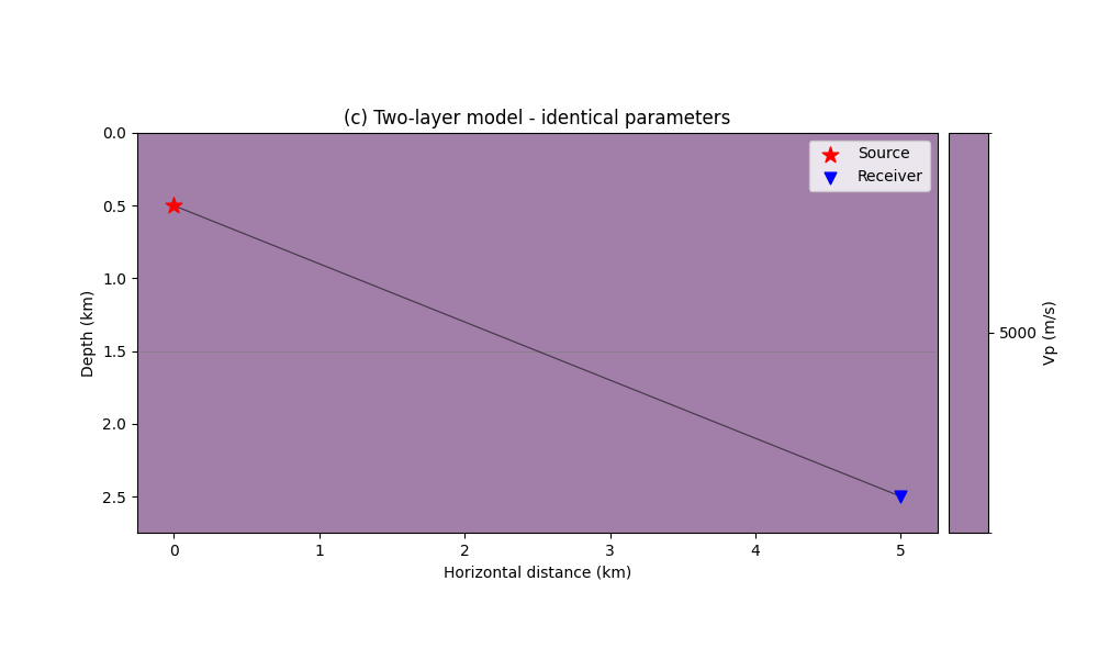
(c) Two-layer model with identical parameters#
The interface at 1500 m splits the medium into two layers, but both share the same properties. A correct implementation should return a transmission coefficient of 1.0 at that interface and identical travel time, \(t^*\), and spreading.
layered_df = pd.DataFrame({
    "Depth": [0.0, 1500.0],
    "Vp":    [VP, VP],
    "Vs":    [VS, VS],
    "Rho":   [RHO, RHO],
    "Qp":    [QP, QP],
    "Qs":    [QS, QS],
})

res_l = lt.trace_rays(
    sources=src,
    receivers=rcv,
    velocity_df=layered_df,
    source_phase="P",
    requested={"travel_times", "rays", "ray_parameters", "tstar", "spreading", "trans_product"},
    transcoef_method="standard",
)

tt_l  = float(res_l.travel_times[0])
p_l   = float(res_l.ray_parameters[0])
ts_l  = float(res_l.tstar[0])
L_l   = float(res_l.spreading[0])
T_l   = float(res_l.trans_product[0])
C_l   = T_l / L_l

print(f"\n--- Layered code (identical layers) ---")
print(f"Travel time:      {tt_l:.8f} s")
print(f"Ray parameter:    {p_l:.10e} s/m")
print(f"t*:               {ts_l:.10e} s")
print(f"Spreading:        {L_l:.4f}")
print(f"Trans. product:   {T_l:.6f}")
print(f"Combined (T/L):   {C_l:.10e}")
--- Layered code (identical layers) ---
Travel time:      1.07703296 s
Ray parameter:    1.8569533818e-04 s/m
t*:               2.1540659229e-03 s
Spreading:        26925824.0357
Trans. product:   1.000000
Combined (T/L):   3.7139067635e-08
Plot the ray through the two-layer model#
The interface at 1500 m is visible, but the ray is identical to the homogeneous case (a straight line) because the two layers share the same velocity.
ax = lt.plot.rays_2d(
    layered_df,
    rays=res_l.rays,
    sources=np.atleast_2d(src),
    receivers=np.atleast_2d(rcv),
    vel_type="Vp",
    add_colorbar=True,
    model_alpha=0.5,
    discrete_colorbar=True,
    unit="km",
)
ax.set_title("(c) Two-layer model - identical parameters")
ax.legend(loc="upper right")
plt.show()
Comparison table#
Collect all results into a DataFrame for easy visual inspection.
labels = [
    "Travel time (s)",
    "Ray parameter (s/m)",
    "t* (s)",
    "Spreading",
    "Trans. product",
    "Combined (T/L)",
]

vals_a = [tt_a, p_a, ts_a, L_a, T_a, C_a]
vals_h = [tt_h, p_h, ts_h, L_h, T_h, C_h]
vals_l = [tt_l, p_l, ts_l, L_l, T_l, C_l]

comparison = pd.DataFrame({
    "(a) Analytical": vals_a,
    "(b) Homo code":  vals_h,
    "(c) Layered code": vals_l,
}, index=labels)

print("\n" + comparison.to_string())
                     (a) Analytical  (b) Homo code  (c) Layered code
Travel time (s)        1.077033e+00   1.077033e+00      1.077033e+00
Ray parameter (s/m)    1.856953e-04   1.856953e-04      1.856953e-04
t* (s)                 2.154066e-03   2.154066e-03      2.154066e-03
Spreading              2.692582e+07   2.692582e+07      2.692582e+07
Trans. product         1.000000e+00   1.000000e+00      1.000000e+00
Combined (T/L)         3.713907e-08   3.713907e-08      3.713907e-08
Relative errors#
Quantify the mismatch between each code result and the analytical reference. Values should be at the machine-precision level.
rel_err_h = np.abs((np.array(vals_h) - np.array(vals_a))
                    / np.where(np.array(vals_a) != 0, vals_a, 1.0))
rel_err_l = np.abs((np.array(vals_l) - np.array(vals_a))
                    / np.where(np.array(vals_a) != 0, vals_a, 1.0))

err_df = pd.DataFrame({
    "Homo vs Analytical": rel_err_h,
    "Layered vs Analytical": rel_err_l,
}, index=labels)

print("\nRelative errors:")
print(err_df.to_string(float_format="{:.2e}".format))
Relative errors:
                     Homo vs Analytical  Layered vs Analytical
Travel time (s)                0.00e+00               6.18e-16
Ray parameter (s/m)            0.00e+00               2.92e-16
t* (s)                         0.00e+00               6.04e-16
Spreading                      0.00e+00               0.00e+00
Trans. product                 0.00e+00               0.00e+00
Combined (T/L)                 0.00e+00               0.00e+00
Accuracy check#
Assert that every quantity agrees across all three approaches to better than \(10^{-10}\) relative tolerance. This is a hard pass/fail gate that can catch regressions.
TOL = 1e-10

def _check(name, ref, val, tol=TOL):
    """Return (name, ref, val, rel_err, status)."""
    if ref == 0:
        err = abs(val)
    else:
        err = abs((val - ref) / ref)
    status = "PASS" if err <= tol else "FAIL"
    return (name, ref, val, err, status)

checks = []
# (b) homo code vs analytical
checks.append(_check("tt   (b) vs (a)", tt_a, tt_h))
checks.append(_check("p    (b) vs (a)", p_a,  p_h))
checks.append(_check("t*   (b) vs (a)", ts_a, ts_h))
checks.append(_check("L    (b) vs (a)", L_a,  L_h))
checks.append(_check("T    (b) vs (a)", T_a,  T_h))
checks.append(_check("C    (b) vs (a)", C_a,  C_h))
# (c) layered code vs analytical
checks.append(_check("tt   (c) vs (a)", tt_a, tt_l))
checks.append(_check("p    (c) vs (a)", p_a,  p_l))
checks.append(_check("t*   (c) vs (a)", ts_a, ts_l))
checks.append(_check("L    (c) vs (a)", L_a,  L_l))
checks.append(_check("T    (c) vs (a)", T_a,  T_l))
checks.append(_check("C    (c) vs (a)", C_a,  C_l))
# (c) layered code vs (b) homo code
checks.append(_check("tt   (c) vs (b)", tt_h, tt_l))
checks.append(_check("p    (c) vs (b)", p_h,  p_l))
checks.append(_check("t*   (c) vs (b)", ts_h, ts_l))
checks.append(_check("L    (c) vs (b)", L_h,  L_l))
checks.append(_check("T    (c) vs (b)", T_h,  T_l))
checks.append(_check("C    (c) vs (b)", C_h,  C_l))

check_df = pd.DataFrame(
    checks, columns=["Check", "Reference", "Value", "Rel. error", "Status"]
)

print(f"\nAccuracy checks (tolerance = {TOL:.0e}):\n")
print(check_df.to_string(index=False, float_format="{:.6e}".format))

n_fail = (check_df["Status"] == "FAIL").sum()
print(f"\nResult: {len(checks) - n_fail}/{len(checks)} checks passed.")
if n_fail:
    print(">>> SOME CHECKS FAILED - investigate! <<<")
else:
    print("All checks passed - homogeneous equivalence confirmed.")
Accuracy checks (tolerance = 1e-10):

          Check    Reference        Value   Rel. error Status
tt   (b) vs (a) 1.077033e+00 1.077033e+00 0.000000e+00   PASS
p    (b) vs (a) 1.856953e-04 1.856953e-04 0.000000e+00   PASS
t*   (b) vs (a) 2.154066e-03 2.154066e-03 0.000000e+00   PASS
L    (b) vs (a) 2.692582e+07 2.692582e+07 0.000000e+00   PASS
T    (b) vs (a) 1.000000e+00 1.000000e+00 0.000000e+00   PASS
C    (b) vs (a) 3.713907e-08 3.713907e-08 0.000000e+00   PASS
tt   (c) vs (a) 1.077033e+00 1.077033e+00 6.184897e-16   PASS
p    (c) vs (a) 1.856953e-04 1.856953e-04 2.919304e-16   PASS
t*   (c) vs (a) 2.154066e-03 2.154066e-03 6.039939e-16   PASS
L    (c) vs (a) 2.692582e+07 2.692582e+07 0.000000e+00   PASS
T    (c) vs (a) 1.000000e+00 1.000000e+00 0.000000e+00   PASS
C    (c) vs (a) 3.713907e-08 3.713907e-08 0.000000e+00   PASS
tt   (c) vs (b) 1.077033e+00 1.077033e+00 6.184897e-16   PASS
p    (c) vs (b) 1.856953e-04 1.856953e-04 2.919304e-16   PASS
t*   (c) vs (b) 2.154066e-03 2.154066e-03 6.039939e-16   PASS
L    (c) vs (b) 2.692582e+07 2.692582e+07 0.000000e+00   PASS
T    (c) vs (b) 1.000000e+00 1.000000e+00 0.000000e+00   PASS
C    (c) vs (b) 3.713907e-08 3.713907e-08 0.000000e+00   PASS

Result: 18/18 checks passed.
All checks passed - homogeneous equivalence confirmed.
Offset-dependent equivalence#
Repeat the comparison for a range of offsets, similarly to example 04, and show that homogeneous and identical-layered models produce overlapping curves for all amplitude-related quantities.
offsets = np.arange(500.0, 15001.0, 500.0)
src_off = np.array([src[0], src[1], rcv[2]])
rcvs = np.column_stack([
    offsets,
    np.zeros_like(offsets),
    np.full_like(offsets, src[2]),
])

res_h_off = lt.trace_rays(
    sources=src_off,
    receivers=rcvs,
    velocity_df=homo_df,
    source_phase="P",
    requested={"travel_times", "rays", "ray_parameters", "tstar", "spreading", "trans_product"},
    transcoef_method="standard",
)

res_l_off = lt.trace_rays(
    sources=src_off,
    receivers=rcvs,
    velocity_df=layered_df,
    source_phase="P",
    requested={"travel_times", "rays", "ray_parameters", "tstar", "spreading", "trans_product"},
    transcoef_method="standard",
)
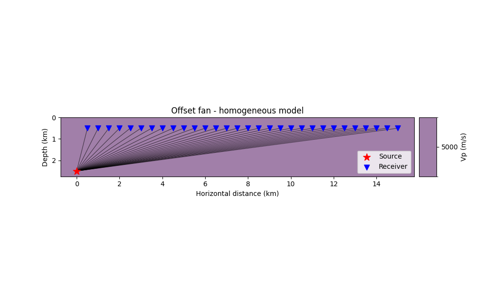
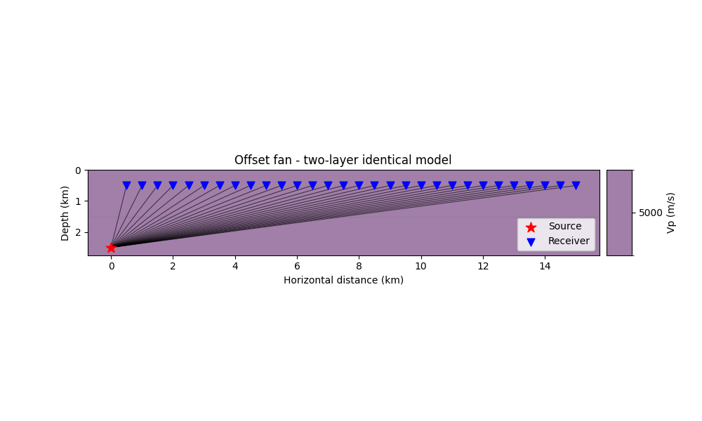
Offset-dependent ray paths#
Plot the full fan of rays for all offsets in both models.
ax = lt.plot.rays_2d(
    homo_df,
    rays=res_h_off.rays,
    sources=np.atleast_2d(src_off),
    receivers=rcvs,
    vel_type="Vp",
    add_colorbar=True,
    model_alpha=0.5,
    discrete_colorbar=True,
    unit="km",
)
ax.set_title("Offset fan - homogeneous model")
ax.legend(loc="lower right")
plt.show()

ax = lt.plot.rays_2d(
    layered_df,
    rays=res_l_off.rays,
    sources=np.atleast_2d(src_off),
    receivers=rcvs,
    vel_type="Vp",
    add_colorbar=True,
    model_alpha=0.5,
    discrete_colorbar=True,
    unit="km",
)
ax.set_title("Offset fan - two-layer identical model")
ax.legend(loc="lower right")
plt.show()

combined_h_off = res_h_off.trans_product / res_h_off.spreading
combined_l_off = res_l_off.trans_product / res_l_off.spreading

curve_relerr = pd.DataFrame({
    "Travel time": np.abs((res_l_off.travel_times - res_h_off.travel_times) / res_h_off.travel_times),
    "t*": np.abs((res_l_off.tstar - res_h_off.tstar) / res_h_off.tstar),
    "Relative Spreading": np.abs((res_l_off.spreading - res_h_off.spreading) / res_h_off.spreading),
    "Trans. product": np.abs((res_l_off.trans_product - res_h_off.trans_product) / np.where(res_h_off.trans_product != 0, res_h_off.trans_product, 1.0)),
    "Combined (T/L)": np.abs((combined_l_off - combined_h_off) / combined_h_off),
}, index=offsets.astype(int))

print("\nMax relative mismatch over offsets (Layered vs Homo):")
print(curve_relerr.max().to_string(float_format="{:.2e}".format))

fig, axes = plt.subplots(3, 2, figsize=(12, 10), sharex=True)
axes = axes.ravel()

km = offsets / 1000.0

axes[0].plot(km, res_h_off.travel_times, "-", linewidth=2, label="Homo")
axes[0].plot(km, res_l_off.travel_times, "--", linewidth=2, label="Layered (identical)")
axes[0].set_ylabel("Travel time (s)")
axes[0].set_title("Travel time")
axes[0].grid(True, alpha=0.3)

axes[1].plot(km, res_h_off.tstar, "-", linewidth=2, label="Homo")
axes[1].plot(km, res_l_off.tstar, "--", linewidth=2, label="Layered (identical)")
axes[1].set_ylabel(r"$t^*$ (s)")
axes[1].set_title(r"Attenuation operator $t^*$")
axes[1].grid(True, alpha=0.3)

axes[2].plot(km, res_h_off.spreading, "-", linewidth=2, label="Homo")
axes[2].plot(km, res_l_off.spreading, "--", linewidth=2, label="Layered (identical)")
axes[2].set_ylabel("Spreading")
axes[2].set_title("Geometrical spreading")
axes[2].grid(True, alpha=0.3)

axes[3].plot(km, res_h_off.trans_product, "-", linewidth=2, label="Homo")
axes[3].plot(km, res_l_off.trans_product, "--", linewidth=2, label="Layered (identical)")
axes[3].set_ylabel(r"$\prod |T_k|$")
axes[3].set_title("Transmission product")
axes[3].grid(True, alpha=0.3)

axes[4].plot(km, combined_h_off, "-", linewidth=2, label="Homo")
axes[4].plot(km, combined_l_off, "--", linewidth=2, label="Layered (identical)")
axes[4].set_ylabel("Combined (T/L)")
axes[4].set_title("Combined deterministic factor")
axes[4].set_xlabel("Offset (km)")
axes[4].grid(True, alpha=0.3)

axes[5].plot(km, res_h_off.ray_parameters, "-", linewidth=2, label="Homo")
axes[5].plot(km, res_l_off.ray_parameters, "--", linewidth=2, label="Layered (identical)")
axes[5].set_ylabel("Ray parameter (s/m)")
axes[5].set_title("Ray parameter")
axes[5].set_xlabel("Offset (km)")
axes[5].grid(True, alpha=0.3)

for ax in axes:
    ax.legend(loc="best")

fig.suptitle("Offset-dependent equivalence: homogeneous vs identical-layered", fontsize=13)
fig.tight_layout()
plt.show()
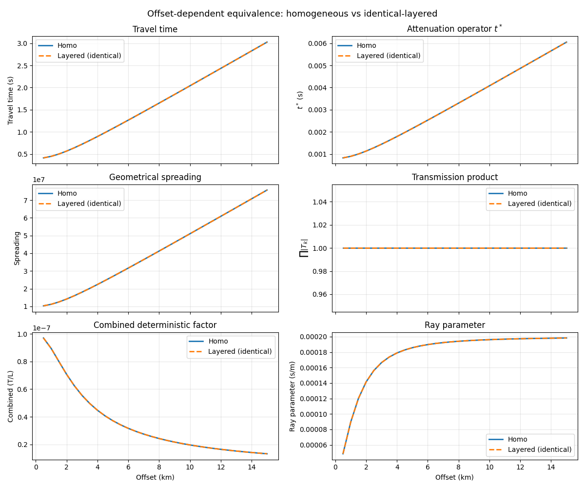
Max relative mismatch over offsets (Layered vs Homo):
Travel time          8.64e-15
t*                   8.74e-15
Relative Spreading   4.43e-15
Trans. product       2.22e-16
Combined (T/L)       4.33e-15
Conclusion#
This extended quality test now validates equivalence at two levels:
Single source-receiver pair: analytical homogeneous formulas, homogeneous code, and identical-layered code agree for travel time, ray parameter, \(t^*\), geometrical spreading, transmission product, and combined factor.
Offset sweep: homogeneous and identical-layered models produce overlapping ray fans and overlapping offset-dependent curves for all computed quantities, with relative mismatches at machine precision.
Therefore, inserting an interface between layers with identical elastic parameters introduces no spurious kinematic or amplitude effects in LayTracer, as required by the underlying physics.
Total running time of the script: (0 minutes 0.749 seconds)