04. Amplitude analysis

This example demonstrates the computation of amplitude-related quantities alongside ray tracing: the attenuation operator \(t^*\), geometrical spreading, and transmission coefficients.

Setup

import laytracer as lt
import numpy as np
import pandas as pd
import matplotlib.pyplot as plt

# sphinx_gallery_thumbnail_number = 2

Define velocity model

vel_df = pd.DataFrame({
    "Depth": [0.0, 1000.0, 2000.0, 3500.0],
    "Vp":    [3000.0, 4500.0, 5500.0, 6500.0],
    "Vs":    [1500.0, 2250.0, 2750.0, 3250.0],
    "Rho":   [2200.0, 2500.0, 2700.0, 2900.0],
    "Qp":    [200.0,  50.0,   600.0,  800.0],
    "Qs":    [100.0,  25.0,   300.0,  400.0],
})

print(vel_df)

    Depth      Vp      Vs     Rho     Qp     Qs
0     0.0  3000.0  1500.0  2200.0  200.0  100.0
1  1000.0  4500.0  2250.0  2500.0   50.0   25.0
2  2000.0  5500.0  2750.0  2700.0  600.0  300.0
3  3500.0  6500.0  3250.0  2900.0  800.0  400.0

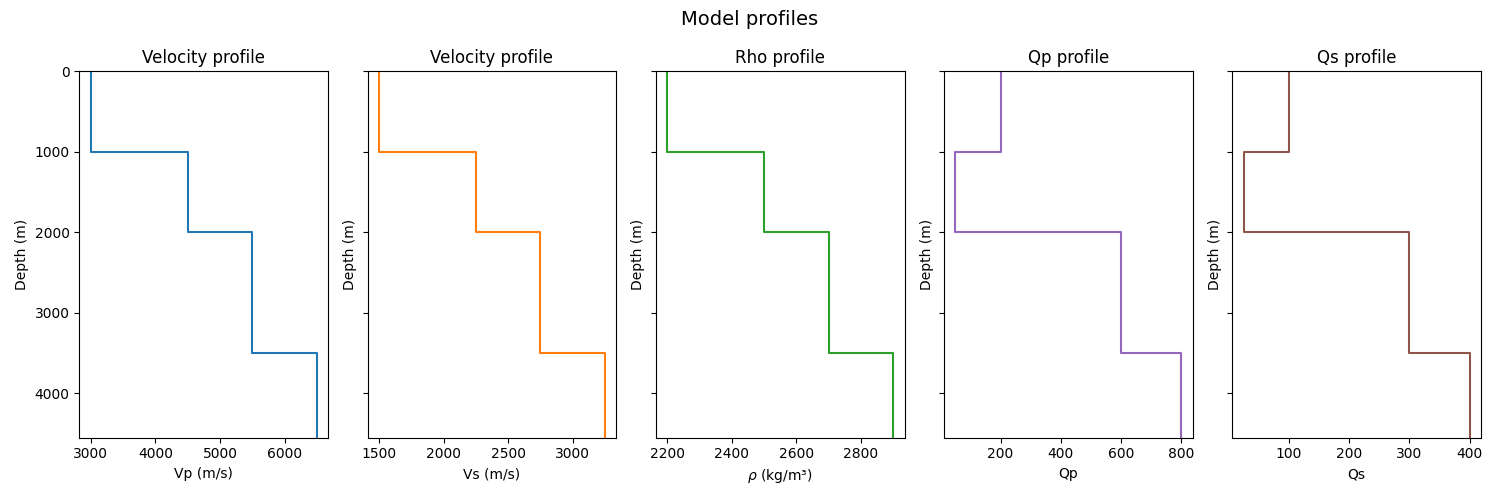
Plot velocity model

Visualise the parameters of the model (P-wave, S-wave, density, attenuation) that will be used for the amplitude calculations.

fig, axes = plt.subplots(1, 5, figsize=(15, 5), sharey=True)

lt.plot.velocity_profile(vel_df, param="Vp", ax=axes[0])
lt.plot.velocity_profile(vel_df, param="Vs", ax=axes[1], color="tab:orange")
lt.plot.velocity_profile(vel_df, param="Rho", ax=axes[2], color="tab:green")
lt.plot.velocity_profile(vel_df, param="Qp", ax=axes[3], color="tab:purple")
lt.plot.velocity_profile(vel_df, param="Qs", ax=axes[4], color="tab:brown")

fig.suptitle("Model profiles", fontsize=14)
fig.tight_layout()
plt.show()

Trace rays with amplitude computation

Trace P-waves from a deep source to receivers at varying offsets, requesting \(t^*\), relative geometrical spreading, and transmission.

src = np.array([0.0, 0.0, 3000.0])

offsets = np.arange(500, 15001, 500)
rcvs = np.column_stack([offsets, np.zeros_like(offsets), np.zeros_like(offsets)])

result = lt.trace_rays(
    sources=src,
    receivers=rcvs,
    velocity_df=vel_df,
    source_phase="P",
    requested={"travel_times", "rays", "ray_parameters", "tstar", "spreading", "trans_product"},
    transcoef_method="standard",
)

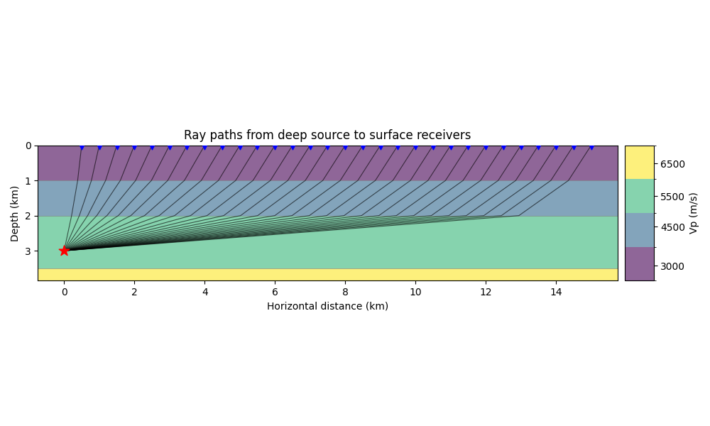
Plot ray paths

Before analysing the amplitudes, let’s visualize the ray paths from the source to the receivers. We overlay the rays on the P-wave velocity model to observe their trajectories.

fig, ax = plt.subplots(figsize=(10, 6))
lt.plot.rays_2d(
    vel_df,
    rays=result.rays,
    sources=src,
    receivers=rcvs,
    ax=ax,
    vel_type="Vp",
    plot_model=True,
    add_colorbar=True,
    model_alpha=0.6,
    discrete_colorbar=True,
    unit="km",
)
ax.set_title("Ray paths from deep source to surface receivers")
fig.tight_layout()
plt.show()

Plot amplitude quantities vs offset

Here we analyze the variation of different amplitude-related quantities as a function of receiver offset:

• Travel time: Increases smoothly with offset. The curvature is governed by the velocity structure (moveout equation).

• Attenuation operator \(t^*\): Calculated as the path integral \(t^* = \int_{\mathrm{ray}} \frac{dt}{Q(s)}\). It represents cumulative anelastic decay. Rays traveling further horizontally spend more time traversing the highly attenuating layer (Q=50) between 1-2 km depth, accumulating higher \(t^*\).

• Geometrical spreading: Measures the spatial divergence of the energetic ray tube. It generally grows with propagation distance, but velocity contrasts distort wavefronts, causing focusing or defocusing effects.

• Transmission coefficient product: The cumulative product of Zoeppritz transmission coefficients \(\prod |T_k|\) across all crossed interfaces. Notice how the transmission efficiency drops sharply at larger offsets as the rays become more grazing, converting more energy into reflected modes.

fig, axes = plt.subplots(2, 2, figsize=(10, 8))

axes[0, 0].plot(offsets / 1000, result.travel_times, "o-", markersize=3)
axes[0, 0].set_xlabel("Offset (km)")
axes[0, 0].set_ylabel("Travel time (s)")
axes[0, 0].set_title("Travel time")
axes[0, 0].grid(True, alpha=0.3)

axes[0, 1].plot(offsets / 1000, result.tstar, "o-", markersize=3, color="tab:orange")
axes[0, 1].set_xlabel("Offset (km)")
axes[0, 1].set_ylabel(r"$t^*$ (s)")
axes[0, 1].set_title(r"Attenuation operator $t^*$")
axes[0, 1].grid(True, alpha=0.3)

if result.spreading is not None:
    valid = result.spreading > 0
    axes[1, 0].plot(
        offsets[valid] / 1000, result.spreading[valid],
        "o-", markersize=3, color="tab:green",
    )
axes[1, 0].set_xlabel("Offset (km)")
axes[1, 0].set_ylabel("Relative spreading factor")
axes[1, 0].set_title("Geometrical spreading")
axes[1, 0].grid(True, alpha=0.3)

axes[1, 1].plot(
    offsets / 1000, result.trans_product,
    "o-", markersize=3, color="tab:red",
)
axes[1, 1].set_xlabel("Offset (km)")
axes[1, 1].set_ylabel(r"$\prod |T_k|$")
axes[1, 1].set_title("Transmission coefficient product")
axes[1, 1].grid(True, alpha=0.3)

fig.suptitle("Amplitude quantities vs. offset", fontsize=14)
fig.tight_layout()
plt.show()

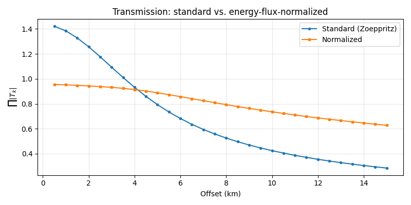
Compare standard vs energy-flux-normalized transmission

The "normalized" method applies the Červený [2001] Eq. 5.3.10 energy-flux normalization to the Zoeppritz coefficients. Normalized coefficients conserve energy flux across each interface, whereas standard (displacement-amplitude) coefficients do not.

result_normalized = lt.trace_rays(
    sources=src,
    receivers=rcvs,
    velocity_df=vel_df,
    source_phase="P",
    requested={"travel_times", "rays", "ray_parameters", "tstar", "spreading", "trans_product"},
    transcoef_method="normalized",
)

fig, ax = plt.subplots(figsize=(8, 4))
ax.plot(offsets / 1000, result.trans_product, "o-", label="Standard (Zoeppritz)", markersize=3)
ax.plot(offsets / 1000, result_normalized.trans_product, "s-", label="Normalized", markersize=3)
ax.set_xlabel("Offset (km)")
ax.set_ylabel(r"$\prod |T_k|$")
ax.set_title("Transmission: standard vs. energy-flux-normalized")
ax.legend()
ax.grid(True, alpha=0.3)
fig.tight_layout()
plt.show()

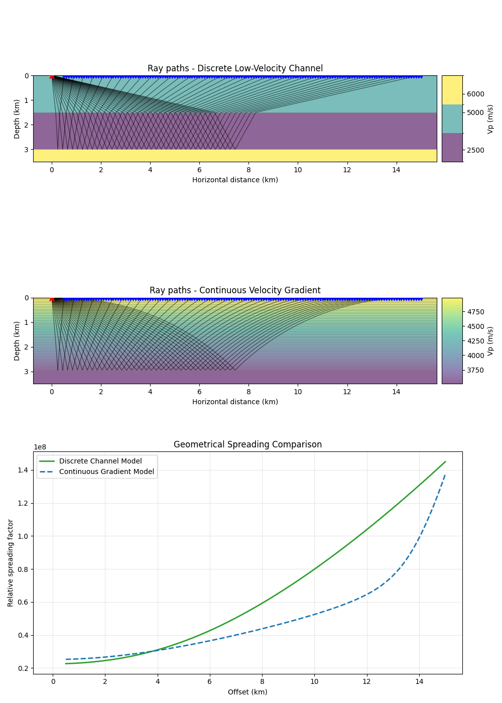
Advanced Spreading Analysis

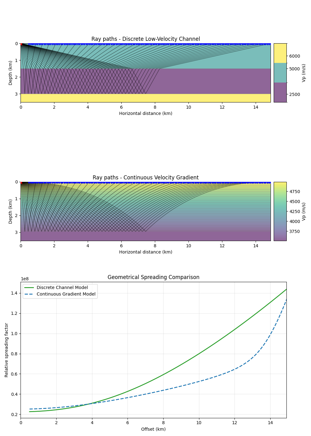
This section compares how different velocity structures (discrete channel vs. continuous gradient) distort the wavefront and influence geometrical spreading.

1. Low-Velocity Channel: Discrete layers funnelling rays.

2. Continuous Gradient: Smoothly varying velocity (discretized).

In flat 1D media, even with strong refraction, geometrical spreading for reflections remains growing and caustic-free.

Comparative Analysis of the Results:

1. Initial Magnitude: The Gradient model (Blue) starts with a higher spreading factor than the Channel model (Green). This is because the average velocity in the gradient (\(5000 \to 3500\) m/s) is higher than in the channel (\(5000 \to 2500\) m/s). Higher average velocity leads to faster initial ray-tube expansion.

2. Curvature & Rate of Change:

   • The Discrete Channel (Green) follows a predictable parabolic growth. The refraction is “lumped” at a single interface, after which the rays travel straight.

   • The Continuous Gradient (Blue) stays “flatter” for mid-offsets but then undergoes an aggressive “upturn” at large offsets (>12 km). This happens because the continuous refraction makes the horizontal offset \(x(p)\) extremely sensitive to changes in take-off angle as rays become grazing.

3. Monotonicity: Importantly, neither curve shows a “dip” or singularity. In 1D flat media, \(dx/dp\) remains positive for reflections, meaning we see no caustics, only varying rates of wavefield divergence.

from laytracer.model import discretize_gradient_layer

# --- 1. Define Models & Trace Rays ---

# Discrete Channel Model
refr_df = pd.DataFrame({
    "Depth": [0.0, 1500.0, 3000.0],
    "Vp":    [5000.0, 2500.0, 6000.0],
    "Vs":    [2880.0, 1440.0, 3460.0],
    "Rho":   [2700.0, 2200.0, 2800.0],
    "Qp":    [300.0,  300.0,  300.0, ],
    "Qs":    [150.0,  150.0,  150.0, ],
})

# Continuous Gradient Model (approximated by 50m layers)
def v_func(z):
    return 5000.0 - 0.5 * z
grad_df = discretize_gradient_layer(0.0, 3000.0, v_func, dz=50.0)

src_p = np.array([0.0, 0.0, 0.0])
offsets = np.arange(500, 15001, 100)
rcvs_p = np.column_stack([offsets, np.zeros_like(offsets), np.zeros_like(offsets)])

# Trace Category 1: Channel
res_refr = lt.trace_rays(
    sources=src_p, receivers=rcvs_p, velocity_df=refr_df,
    source_phase="P", reflection=[(3000.0, "P")],
    requested={"travel_times", "rays", "ray_parameters", "tstar", "spreading", "trans_product"}, transcoef_method="standard"
)

# Trace Category 2: Gradient (reflect off last interface ~3km)
z_reflect = grad_df["Depth"].iloc[-1]
res_grad = lt.trace_rays(
    sources=src_p, receivers=rcvs_p, velocity_df=grad_df,
    source_phase="P", reflection=[(z_reflect, "P")],
    requested={"travel_times", "rays", "ray_parameters", "tstar", "spreading", "trans_product"}, transcoef_method="standard"
)

# --- 2. Advanced Visualisation ---

fig, (ax1, ax2, ax3) = plt.subplots(3, 1, figsize=(10, 14), sharex=True)

# Panel 1: Channel Rays
lt.plot.rays_2d(
    refr_df, rays=res_refr.rays[::4],
    sources=src_p, receivers=rcvs_p, ax=ax1,
    vel_type="Vp", model_alpha=0.6,
    plot_model=True, add_colorbar=True, discrete_colorbar=True, unit="km",
)
ax1.set_title("Ray paths - Discrete Low-Velocity Channel")
ax1.set_ylim(3.5, 0)
ax1.tick_params(labelbottom=True) # Forces x-labels to show despite sharex=True

# Panel 2: Gradient Rays
lt.plot.rays_2d(
    grad_df, rays=res_grad.rays[::4],
    sources=src_p, receivers=rcvs_p, ax=ax2,
    vel_type="Vp", model_alpha=0.6,
    plot_model=True, add_colorbar=True, discrete_colorbar=False, unit="km",
)
ax2.set_title("Ray paths - Continuous Velocity Gradient")
ax2.set_ylim(3.5, 0)
ax2.tick_params(labelbottom=True)


# Panel 3: Spreading Comparison
valid_f = res_refr.spreading > 0
valid_g = res_grad.spreading > 0

ax3.plot(
    offsets[valid_f] / 1000, res_refr.spreading[valid_f],
    "-", color="tab:green", label="Discrete Channel Model", linewidth=2
)
ax3.plot(
    offsets[valid_g] / 1000, res_grad.spreading[valid_g],
    "--", color="tab:blue", label="Continuous Gradient Model", linewidth=2
)

ax3.set_xlabel("Offset (km)")
ax3.set_ylabel("Relative spreading factor")
ax3.set_title("Geometrical Spreading Comparison")
ax3.legend()
ax3.grid(True, alpha=0.3)

plt.tight_layout()
plt.show()

References

[1]

V. Červený. Seismic Ray Theory. Cambridge University Press, 2001. doi:10.1017/CBO9780511529399.