03. Reflection & transmission

Reproduction of the classic P-SV reflection & transmission test case from Charles J. Ammon’s MATLAB Exercise L3 (PDF) (Lay and Wallace [1995], Figure 3.28). The example also includes the decoupled SH-SH coefficients for the same two-layer elastic model.

For an incident P-wave the system unknowns are \([R_{PP},\; R_{PS},\; T_{PP},\; T_{PS}]\). For an incident SV-wave the unknowns are \([R_{SP},\; R_{SS},\; T_{SP},\; T_{SS}]\). For an incident SH-wave the unknowns are \([R_{SHSH},\; T_{SHSH}]\).

Setup

import laytracer as lt
import numpy as np
import pandas as pd
import matplotlib.pyplot as plt

# sphinx_gallery_thumbnail_number = 2

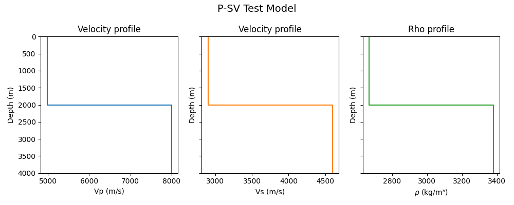
Model

Medium parameters (Km/s and g/cm^3)

mi_vp, mi_vs, mi_rho = 4.98, 2.9, 2.667   # incident
mt_vp, mt_vs, mt_rho = 8.00, 4.6, 3.38    # transmitted

# Create a DataFrame for visualization (using SI units m/s, kg/m^3)
model_psv = pd.DataFrame({
    "Depth": [0.0, 2000.0],  # Arbitrary interface depth at 2km
    "Vp":    [mi_vp * 1000, mt_vp * 1000],
    "Vs":    [mi_vs * 1000, mt_vs * 1000],
    "Rho":   [mi_rho * 1000, mt_rho * 1000],
})

# Plot the velocity model
fig, axes = plt.subplots(1, 3, figsize=(10, 4), sharey=True)
lt.plot.velocity_profile(model_psv, param="Vp", ax=axes[0], ylim=(4000, 0))
lt.plot.velocity_profile(model_psv, param="Vs", ax=axes[1], color="tab:orange", ylim=(4000, 0))
lt.plot.velocity_profile(model_psv, param="Rho", ax=axes[2], color="tab:green", ylim=(4000, 0))

fig.suptitle("Elastic Test Model", fontsize=14)
fig.tight_layout()
plt.show()


def _marker_spec(angle, label, color, linestyle, linewidth=0.8):
    return {
        "angle": angle,
        "label": label,
        "line_kwargs": {
            "color": color,
            "ls": linestyle,
            "lw": linewidth,
        },
    }


def _outgoing_evanescent_masks(p, velocities):
    p = np.asarray(p)
    return {
        key: p * velocity > 1.0
        for key, velocity in velocities.items()
    }


ACCENT7 = ("#7fc97f", "#beaed4", "#fdc086", "#ffff99", "#386cb0", "#f0027f", "#bf5b17")
LAYER_COLORS = ACCENT7[3:1:-1]
RAY_COLORS = {
    "Refl P": ACCENT7[4],
    "Refl SV": ACCENT7[1],
    "Trans P": ACCENT7[6],
    "Trans SV": ACCENT7[5],
    "Refl SH": ACCENT7[1],
    "Trans SH": ACCENT7[5],
    "Inc P": ACCENT7[0],
    "Inc SV": ACCENT7[0],
    "Inc SH": ACCENT7[0],
}
RAY_LINEWIDTH = 1.5
RAY_XLIM = (0, 6000)
RAY_YLIM = (4000, 0)


def _coefficient_panels(
    panel_defs,
    curve_defs,
    common_markers,
    panel_markers,
    ylim,
    evanescent_masks=None,
):
    panels = []
    for key, ylabel, title in panel_defs:
        curves = []
        for curve_def in curve_defs:
            coefficient = curve_def["data"][key]
            curve = {
                "y": np.abs(coefficient),
                "complex_from": coefficient,
                "label": curve_def.get("label"),
                "plot_kwargs": dict(curve_def["plot_kwargs"]),
            }
            if evanescent_masks is not None:
                curve["evanescent_mask"] = evanescent_masks.get(key)
            curves.append(curve)

        markers = [dict(marker) for marker in common_markers]
        markers.extend(panel_markers.get(key, []))

        panels.append(
            {
                "curves": curves,
                "markers": markers,
                "title": title,
                "ylabel": ylabel,
                "ylim": ylim,
                "legend": True,
            }
        )

    return panels

# Ray-parameter sweep: p from 0 to 1/Vp_incident
n_p = 1000
p_vec = np.linspace(0, 1.0 / mi_vp, n_p + 1)
evanescent_masks_P = _outgoing_evanescent_masks(
    p_vec,
    {
        "Rpp": mi_vp,
        "Rps": mi_vs,
        "Tpp": mt_vp,
        "Tps": mt_vs,
    },
)

# Compute all 8 R/T coefficients
RT = lt.psv_rt_coefficients(
    p=p_vec,
    vp1=mi_vp, vs1=mi_vs, rho1=mi_rho,
    vp2=mt_vp, vs2=mt_vs, rho2=mt_rho,
)

# In the coefficient panels below, dashed curve segments mark coefficients
# that have become complex while the plotted outgoing branch still propagates.
# Dash-dot curve segments mark the stronger condition where that outgoing
# branch itself has imaginary vertical slowness and is evanescent.

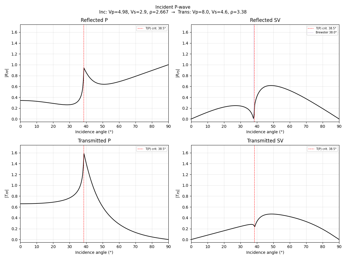
Incident P-wave coefficients

For an incident P-wave the ray parameter sweeps from 0 to \(1/V_P\) (grazing P incidence), covering the full \(0--90^{\circ}\) range.

Critical angle (dashed red line):

• Transmitted P becomes evanescent at \(\theta_c^{T(P)} = \arcsin(V_P^{(1)}/V_P^{(2)}) \approx 38.5^{\circ}\). Beyond this angle the transmitted-P vertical slowness is imaginary, the affected displacement coefficients become complex, and \(|R_{PP}| \to 1\) (total reflection). There is no transmitted-SV critical angle because \(V_P^{(1)} > V_S^{(2)}\) for this model.

Brewster angles (dotted purple lines):

• \(|R_{PS}|\) has a near-zero at \(37.9^{\circ}\), just before the critical angle. This is the P-to-SV mode-conversion null, analogous to the optical Brewster angle. Its position depends on all six elastic parameters, not just the velocity ratio.

# Incidence angle (P-wave): :math:`\theta` = \arcsin{p \cdot V_p}`
angle_P = np.rad2deg(np.arcsin(np.clip(p_vec * mi_vp, -1, 1)))
crit_P = lt.find_critical_angles(mi_vp, {"T(P)": mt_vp})

# Detect Brewster angles for all P-incident coefficients
brew_P = lt.find_brewster_angles(RT, angle_P, keys=["Rpp", "Rps", "Tpp", "Tps"])

# Shared y-limit across all four P-incident panels
p_keys = ["Rpp", "Rps", "Tpp", "Tps"]
ymax_P = max(np.nanmax(np.abs(RT[k])) for k in p_keys) * 1.1
ymax_P = max(ymax_P, 0.5)

labels = [
    ("Rpp", r"$|R_{PP}|$", "Reflected P"),
    ("Rps", r"$|R_{PS}|$", "Reflected SV"),
    ("Tpp", r"$|T_{PP}|$", "Transmitted P"),
    ("Tps", r"$|T_{PS}|$", "Transmitted SV"),
]
common_markers_P = [
    _marker_spec(
        crit_P["T(P)"],
        f"T(P) crit. {crit_P['T(P)']:.1f} deg",
        "r",
        "--",
    )
]
panel_markers_P = {
    key: [
        _marker_spec(ba, f"Brewster {ba:.1f} deg", "tab:purple", ":")
        for ba in brew_P.get(key, [])
    ]
    for key in p_keys
}
panels = _coefficient_panels(
    labels,
    curve_defs=[{"data": RT, "plot_kwargs": {"color": "k", "lw": 1.5}}],
    common_markers=common_markers_P,
    panel_markers=panel_markers_P,
    ylim=(-0.05, ymax_P),
    evanescent_masks=evanescent_masks_P,
)
fig, axes = lt.plot.coefficient_panels(
    panels,
    shape=(2, 2),
    figsize=(12, 9),
    default_x=angle_P,
    default_xlim=(0.0, 90.0),
    default_xlabel="Incidence angle (deg)",
    suptitle=(
        "Incident P-wave\n"
        f"Inc: Vp={mi_vp}, Vs={mi_vs}, rho={mi_rho}  ->  "
        f"Trans: Vp={mt_vp}, Vs={mt_vs}, rho={mt_rho}"
    ),
)
plt.show()

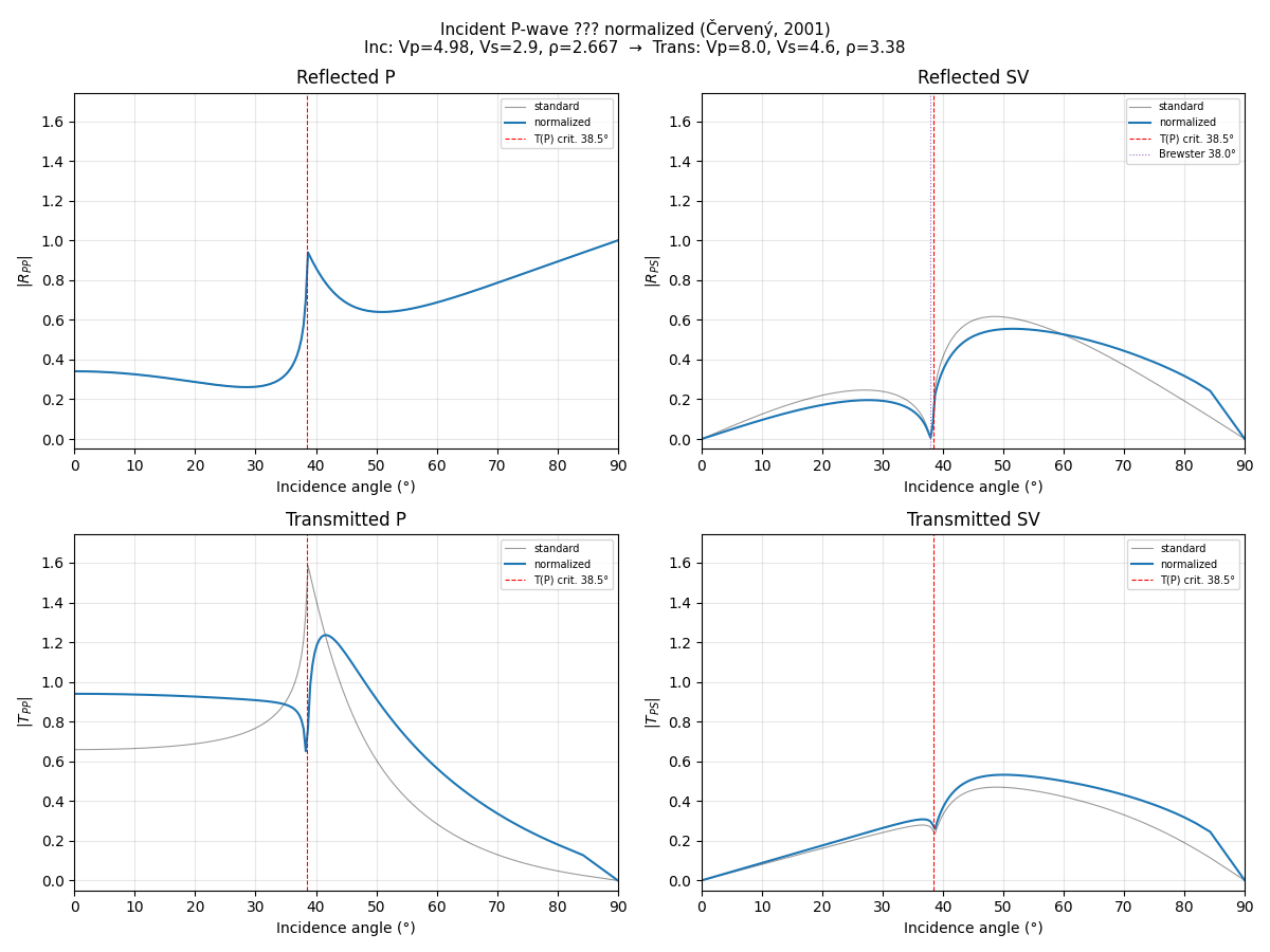
Normalized P-wave coefficients

Energy-flux-normalized coefficients account for the impedance and directional cosine contrast across the interface. They are useful for amplitude-preserving modelling because the product of normalized transmission coefficients along a ray is the displacement-amplitude transfer factor that conserves energy flux.

The normalization follows Červený [2001] Eq. 5.3.10:

\[R_{mn}^\text{norm} = \bar{R}_{mn} \sqrt{\frac{V_{\text{out}}\,\rho_{\text{out}}\, \cos\theta_{\text{out}}} {V_{\text{in}}\,\rho_{\text{in}}\, \cos\theta_{\text{in}}}}\]

# Mapping: key -> (v_in, rho_in, v_out, rho_out)
norm_map_P = {
    "Rpp": (mi_vp, mi_rho, mi_vp, mi_rho),
    "Rps": (mi_vp, mi_rho, mi_vs, mi_rho),
    "Tpp": (mi_vp, mi_rho, mt_vp, mt_rho),
    "Tps": (mi_vp, mi_rho, mt_vs, mt_rho),
}

RT_norm_P = {}
for key, (vi, ri, vo, ro) in norm_map_P.items():
    RT_norm_P[key] = lt.normalize_rt_coefficient(
        RT[key], p_vec, vi, ri, vo, ro,
    )

ymax_Pn = max(
    np.nanmax(np.abs(RT_norm_P[k])) for k in p_keys
) * 1.1
ymax_Pn = max(ymax_Pn, 0.5)

panels = _coefficient_panels(
    labels,
    curve_defs=[
        {
            "data": RT,
            "label": "standard",
            "plot_kwargs": {"color": "k", "lw": 0.8, "alpha": 0.4},
        },
        {
            "data": RT_norm_P,
            "label": "normalized",
            "plot_kwargs": {"color": "tab:blue", "lw": 1.5},
        },
    ],
    common_markers=common_markers_P,
    panel_markers=panel_markers_P,
    ylim=(-0.05, max(ymax_P, ymax_Pn)),
    evanescent_masks=evanescent_masks_P,
)
fig, axes = lt.plot.coefficient_panels(
    panels,
    shape=(2, 2),
    figsize=(12, 9),
    default_x=angle_P,
    default_xlim=(0.0, 90.0),
    default_xlabel="Incidence angle (deg)",
    suptitle=(
        "Incident P-wave - normalized\n"
        f"Inc: Vp={mi_vp}, Vs={mi_vs}, rho={mi_rho}  ->  "
        f"Trans: Vp={mt_vp}, Vs={mt_vs}, rho={mt_rho}"
    ),
)
plt.show()

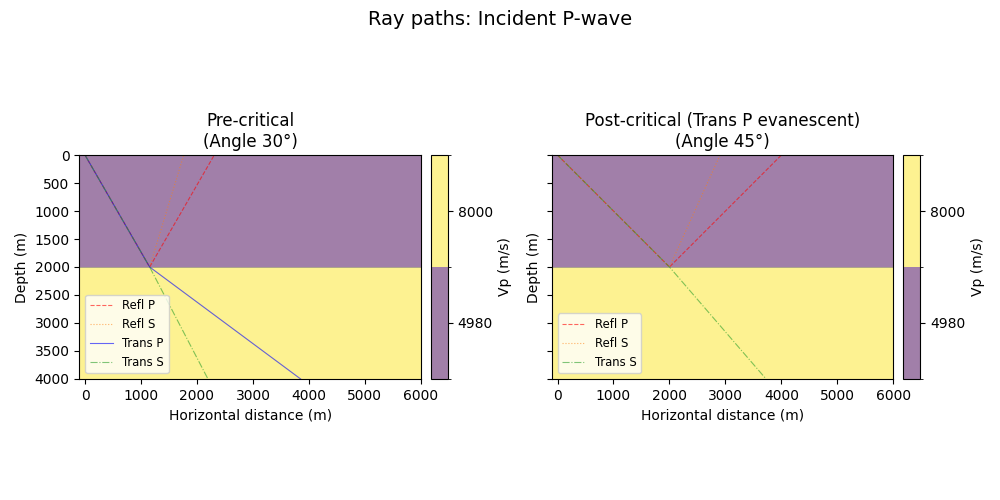
Ray diagrams (P-incidence)

We visualize the ray paths for typical situations using lt.plot.rays_2d. The interface is at 2000 m.

def plot_ray_situation(angle, wave_type, title, ax):
    wave_type = "SV" if wave_type == "S" else wave_type
    shear_phase = wave_type in {"SV", "SH"}

    lt.plot.rays_2d(
        model_psv, rays=[], ax=ax, vel_type="Vs" if shear_phase else "Vp",
        xlim=RAY_XLIM, ylim=RAY_YLIM,
        plot_model=True,
        add_colorbar=True,
        discrete_colorbar=True,
        layer_colors=LAYER_COLORS,
    )

    v_inc = mi_vp * 1000 if wave_type == "P" else mi_vs * 1000
    p_target = np.sin(np.deg2rad(angle)) / v_inc

    source = np.array([[0.0, 0.0, 0.0]])
    z_int = 2000.0
    z_bot = 4000.0

    def phase_velocity(phase, transmitted=False):
        if phase == "P":
            return (mt_vp if transmitted else mi_vp) * 1000
        return (mt_vs if transmitted else mi_vs) * 1000

    def leg_offset(thickness, velocity):
        pv = p_target * velocity
        if pv >= 1.0:
            return None
        return thickness * pv / np.sqrt(1.0 - pv**2)

    def plot_ray_path(ray, label, color):
        lt.plot.rays_2d(
            model_psv,
            rays=[ray],
            ax=ax,
            ray_color=color,
            ray_alpha=1.0,
            ray_linewidth=RAY_LINEWIDTH,
            plot_model=False,
            linestyle="-",
            label=label,
            xlim=RAY_XLIM, ylim=RAY_YLIM,
        )

    dx0 = leg_offset(z_int, phase_velocity(wave_type))
    if dx0 is None:
        ax.set_title(f"{title}\n(Angle {angle:g} deg)")
        return

    incident_ray = np.array([
        [0.0, 0.0, 0.0],
        [dx0, 0.0, z_int],
    ])
    plot_ray_path(incident_ray, f"Inc {wave_type}", RAY_COLORS[f"Inc {wave_type}"])

    def run_trace(reflection_arg=None, refraction_arg=None, label="", color=""):
        if reflection_arg is not None:
            outgoing_phase = reflection_arg[0][1]
            dx1 = leg_offset(z_int, phase_velocity(outgoing_phase))
            z_end = 0.0
        else:
            outgoing_phase = refraction_arg[0][1] if refraction_arg else wave_type
            dx1 = leg_offset(
                z_bot - z_int,
                phase_velocity(outgoing_phase, transmitted=True),
            )
            z_end = z_bot

        if dx1 is None:
            return

        receiver = np.array([[dx0 + dx1, 0.0, z_end]])
        res = lt.trace_rays(
            sources=source,
            receivers=receiver,
            velocity_df=model_psv,
            source_phase=wave_type,
            reflection=reflection_arg,
            refraction=refraction_arg,
            requested={"travel_times", "rays", "ray_parameters"},
        )

        if res.rays and res.rays[0] is not None:
            ray = res.rays[0].copy()
            ray[:, 0] -= ray[0, 0]
            ray[:, 2] -= ray[0, 2]
            outgoing_ray = ray[1:]
            if len(outgoing_ray) >= 2:
                plot_ray_path(outgoing_ray, label, color)

    if wave_type == "SH":
        ray_variants = [
            dict(
                reflection_arg=[(z_int, "SH")],
                label="Refl SH",
                color=RAY_COLORS["Refl SH"],
            ),
            dict(refraction_arg=None, label="Trans SH", color=RAY_COLORS["Trans SH"]),
        ]
    elif wave_type == "P":
        ray_variants = [
            dict(
                reflection_arg=[(z_int, "P")],
                label="Refl P",
                color=RAY_COLORS["Refl P"],
            ),
            dict(
                reflection_arg=[(z_int, "SV")],
                label="Refl SV",
                color=RAY_COLORS["Refl SV"],
            ),
            dict(refraction_arg=None, label="Trans P", color=RAY_COLORS["Trans P"]),
            dict(
                refraction_arg=[(z_int, "SV")],
                label="Trans SV",
                color=RAY_COLORS["Trans SV"],
            ),
        ]
    else:
        ray_variants = [
            dict(
                reflection_arg=[(z_int, "P")],
                label="Refl P",
                color=RAY_COLORS["Refl P"],
            ),
            dict(
                reflection_arg=[(z_int, "SV")],
                label="Refl SV",
                color=RAY_COLORS["Refl SV"],
            ),
            dict(refraction_arg=[(z_int, "P")], label="Trans P", color=RAY_COLORS["Trans P"]),
            dict(refraction_arg=None, label="Trans SV", color=RAY_COLORS["Trans SV"]),
        ]

    for variant in ray_variants:
        run_trace(**variant)

    ax.legend(loc="upper right", fontsize="small")
    ax.set_title(f"{title}\n(Angle {angle:g} deg)")


def show_ray_subplot_labels(axes):
    for ax in np.ravel(axes):
        ax.tick_params(labelbottom=True, labelleft=True)
        ax.set_xlabel("Horizontal distance (m)")
        ax.set_ylabel("Depth (m)")


# P-incidence scenarios
scenarios_p = [
    (30, "Pre-critical"),
    (45, "Post-critical (Trans P evanescent)"),
]

fig, axes = plt.subplots(1, 2, figsize=(10, 5), sharey=True)
for i, (ang, name) in enumerate(scenarios_p):
    plot_ray_situation(ang, "P", name, axes[i])

show_ray_subplot_labels(axes)
fig.suptitle("Ray paths: Incident P-wave", fontsize=14)
fig.tight_layout()
plt.show()

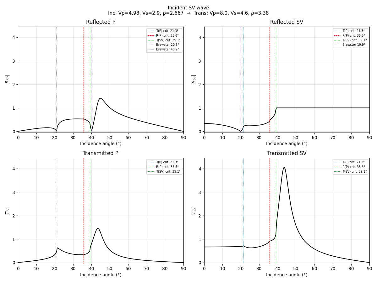
Incident SV-wave coefficients

For an incident SV-wave the ray parameter sweeps from 0 to \(1/V_S\) (grazing SV incidence), covering the full \(0--90^{\circ}\) range.

Critical angles (coloured lines) - three distinct thresholds:

• \(\theta_c^{T(P)} = \arcsin(V_S^{(1)}/V_P^{(2)}) \approx 21.3^{\circ}\) - transmitted P goes evanescent (blue dotted)

• \(\theta_c^{R(P)} = \arcsin(V_S^{(1)}/V_P^{(1)}) \approx 35.6^{\circ}\) - reflected P goes evanescent (red dashed)

• \(\theta_c^{T(SV)} = \arcsin(V_S^{(1)}/V_S^{(2)}) \approx 39.1^{\circ}\) - transmitted SV goes evanescent (green dash-dot); beyond this angle all energy is reflected as SV (\(|R_{SS}| = 1\)).

Once one of these P-SV branches is post-critical, its vertical slowness is imaginary and the coupled Zoeppritz coefficients can become complex. The reflected SV wave remains propagating (same medium, same velocity), but its coefficient can still carry a complex phase from the coupled boundary conditions.

Brewster angles (purple dotted lines) - the near-zeros of \(|R_{SP}|\) near 21° and 40°, and of \(|R_{SS}|\) near 20°, are mode-conversion nulls governed by the full elastic contrast.

p_vec_sv = np.linspace(0, 1.0 / mi_vs, n_p + 1)
evanescent_masks_SV = _outgoing_evanescent_masks(
    p_vec_sv,
    {
        "Rsp": mi_vp,
        "Rss": mi_vs,
        "Tsp": mt_vp,
        "Tss": mt_vs,
    },
)

RT_sv = lt.psv_rt_coefficients(
    p=p_vec_sv,
    vp1=mi_vp, vs1=mi_vs, rho1=mi_rho,
    vp2=mt_vp, vs2=mt_vs, rho2=mt_rho,
)

# Incidence angle (SV-wave):  :math:`\theta = \arcsin(p \cdot V_s)`
angle_SV = np.rad2deg(np.arcsin(np.clip(p_vec_sv * mi_vs, -1, 1)))

# Critical angles
crit_SV = lt.find_critical_angles(
    mi_vs,
    {"T(P)": mt_vp, "R(P)": mi_vp, "T(SV)": mt_vs},
)

# Detect Brewster angles for all SV-incident coefficients
brew_SV = lt.find_brewster_angles(
    RT_sv, angle_SV, keys=["Rsp", "Rss", "Tsp", "Tss"],
)

labels_sv = [
    ("Rsp", r"$|R_{SP}|$", "Reflected P"),
    ("Rss", r"$|R_{SS}|$", "Reflected SV"),
    ("Tsp", r"$|T_{SP}|$", "Transmitted P"),
    ("Tss", r"$|T_{SS}|$", "Transmitted SV"),
]

# Shared y-limit across all four SV-incident panels
sv_keys = ["Rsp", "Rss", "Tsp", "Tss"]
ymax_SV = max(np.nanmax(np.abs(RT_sv[k])) for k in sv_keys) * 1.1
ymax_SV = max(ymax_SV, 0.5)

common_markers_SV = [
    _marker_spec(crit_SV["T(P)"], f"T(P) crit. {crit_SV['T(P)']:.1f} deg", "tab:blue", ":"),
    _marker_spec(crit_SV["R(P)"], f"R(P) crit. {crit_SV['R(P)']:.1f} deg", "r", "--"),
    _marker_spec(crit_SV["T(SV)"], f"T(SV) crit. {crit_SV['T(SV)']:.1f} deg", "tab:green", "-."),
]
panel_markers_SV = {
    key: [
        _marker_spec(ba, f"Brewster {ba:.1f} deg", "tab:purple", ":")
        for ba in brew_SV.get(key, [])
    ]
    for key in sv_keys
}
panels = _coefficient_panels(
    labels_sv,
    curve_defs=[{"data": RT_sv, "plot_kwargs": {"color": "k", "lw": 1.5}}],
    common_markers=common_markers_SV,
    panel_markers=panel_markers_SV,
    ylim=(-0.05, ymax_SV),
    evanescent_masks=evanescent_masks_SV,
)
fig, axes = lt.plot.coefficient_panels(
    panels,
    shape=(2, 2),
    figsize=(12, 9),
    default_x=angle_SV,
    default_xlim=(0.0, 90.0),
    default_xlabel="Incidence angle (deg)",
    suptitle=(
        "Incident SV-wave\n"
        f"Inc: Vp={mi_vp}, Vs={mi_vs}, rho={mi_rho}  ->  "
        f"Trans: Vp={mt_vp}, Vs={mt_vs}, rho={mt_rho}"
    ),
)
plt.show()

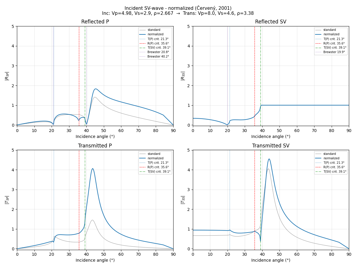
Normalized SV-wave coefficients

Same energy-flux normalization applied to the SV-incident coefficients. The three critical-angle markers are preserved.

# Mapping: key -> (v_in, rho_in, v_out, rho_out)
norm_map_SV = {
    "Rsp": (mi_vs, mi_rho, mi_vp, mi_rho),
    "Rss": (mi_vs, mi_rho, mi_vs, mi_rho),
    "Tsp": (mi_vs, mi_rho, mt_vp, mt_rho),
    "Tss": (mi_vs, mi_rho, mt_vs, mt_rho),
}

RT_norm_SV = {}
for key, (vi, ri, vo, ro) in norm_map_SV.items():
    RT_norm_SV[key] = lt.normalize_rt_coefficient(
        RT_sv[key], p_vec_sv, vi, ri, vo, ro,
    )

ymax_SVn = max(
    np.nanmax(np.abs(RT_norm_SV[k])) for k in sv_keys
) * 1.1
ymax_SVn = max(ymax_SVn, 0.5)

panels = _coefficient_panels(
    labels_sv,
    curve_defs=[
        {
            "data": RT_sv,
            "label": "standard",
            "plot_kwargs": {"color": "k", "lw": 0.8, "alpha": 0.4},
        },
        {
            "data": RT_norm_SV,
            "label": "normalized",
            "plot_kwargs": {"color": "tab:blue", "lw": 1.5},
        },
    ],
    common_markers=common_markers_SV,
    panel_markers=panel_markers_SV,
    ylim=(-0.05, max(ymax_SV, ymax_SVn)),
    evanescent_masks=evanescent_masks_SV,
)
fig, axes = lt.plot.coefficient_panels(
    panels,
    shape=(2, 2),
    figsize=(12, 9),
    default_x=angle_SV,
    default_xlim=(0.0, 90.0),
    default_xlabel="Incidence angle (deg)",
    suptitle=(
        "Incident SV-wave - normalized\n"
        f"Inc: Vp={mi_vp}, Vs={mi_vs}, rho={mi_rho}  ->  "
        f"Trans: Vp={mt_vp}, Vs={mt_vs}, rho={mt_rho}"
    ),
)
plt.show()

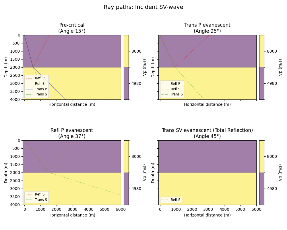
Ray diagrams (SV-incidence)

# SV-incidence scenarios
scenarios_sv = [
    (15, "Pre-critical"),
    (25, "Trans P evanescent"),
    (37, "Refl P evanescent"),
    (45, "Trans SV evanescent (Total Reflection)"),
]

fig, axes = plt.subplots(2, 2, figsize=(10, 8), sharey=True, sharex=True)
axes = axes.flatten()

for i, (ang, name) in enumerate(scenarios_sv):
    plot_ray_situation(ang, "SV", name, axes[i])

show_ray_subplot_labels(axes)
fig.suptitle("Ray paths: Incident SV-wave", fontsize=14)
fig.tight_layout()
plt.show()

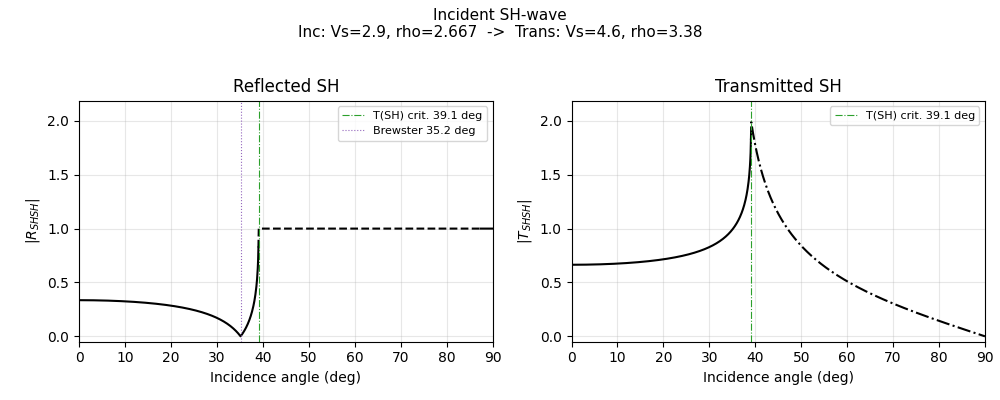
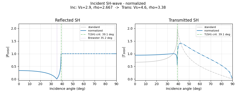
Incident SH-wave coefficients

SH motion is decoupled from P-SV motion in an isotropic 1-D model, so the interface response contains only same-mode reflection and transmission: \(R_{SHSH}\) and \(T_{SHSH}\). The ray-parameter sweep uses the same incident S-wave slowness range as the SV case. The ray diagrams below show the radial-vertical incidence-plane geometry; SH particle motion is polarized perpendicular to that plane.

Critical angle (green dash-dot line):

• \(\theta_c^{T(SH)} = \arcsin(V_S^{(1)}/V_S^{(2)}) \approx 39.1^{\circ}\). Beyond this angle the transmitted-SH vertical slowness is imaginary, so the SH reflection and transmission coefficients are complex while the reflected-SH magnitude stays at total reflection.

SH Brewster/null angle (purple dotted line):

• \(|R_{SHSH}|\) vanishes near \(35.2^{\circ}\) where the oblique SH impedances on both sides match, \(\zeta_1 = \zeta_2\) with \(\zeta_i = \rho_i V_{Si}^2 \eta_i\).

p_vec_sh = np.linspace(0, 1.0 / mi_vs, n_p + 1)
evanescent_masks_SH = _outgoing_evanescent_masks(
    p_vec_sh,
    {
        "Rshsh": mi_vs,
        "Tshsh": mt_vs,
    },
)

RT_sh = lt.sh_rt_coefficients(
    p=p_vec_sh,
    vs1=mi_vs, rho1=mi_rho,
    vs2=mt_vs, rho2=mt_rho,
)

angle_SH = np.rad2deg(np.arcsin(np.clip(p_vec_sh * mi_vs, -1, 1)))
crit_SH = lt.find_critical_angles(mi_vs, {"T(SH)": mt_vs})
brew_SH = lt.find_brewster_angles(RT_sh, angle_SH, keys=["Rshsh"])

labels_sh = [
    ("Rshsh", r"$|R_{SHSH}|$", "Reflected SH"),
    ("Tshsh", r"$|T_{SHSH}|$", "Transmitted SH"),
]
sh_keys = ["Rshsh", "Tshsh"]
ymax_SH = max(np.nanmax(np.abs(RT_sh[k])) for k in sh_keys) * 1.1
ymax_SH = max(ymax_SH, 0.5)

common_markers_SH = [
    _marker_spec(
        crit_SH.get("T(SH)"),
        f"T(SH) crit. {crit_SH['T(SH)']:.1f} deg",
        "tab:green",
        "-.",
    )
]
panel_markers_SH = {
    "Rshsh": [
        _marker_spec(ba, f"Brewster {ba:.1f} deg", "tab:purple", ":")
        for ba in brew_SH.get("Rshsh", [])
    ]
}
panels = _coefficient_panels(
    labels_sh,
    curve_defs=[{"data": RT_sh, "plot_kwargs": {"color": "k", "lw": 1.5}}],
    common_markers=common_markers_SH,
    panel_markers=panel_markers_SH,
    ylim=(-0.05, ymax_SH),
    evanescent_masks=evanescent_masks_SH,
)
fig, axes = lt.plot.coefficient_panels(
    panels,
    shape=(1, 2),
    figsize=(10, 4),
    default_x=angle_SH,
    default_xlim=(0.0, 90.0),
    default_xlabel="Incidence angle (deg)",
    suptitle=(
        "Incident SH-wave\n"
        f"Inc: Vs={mi_vs}, rho={mi_rho}  ->  "
        f"Trans: Vs={mt_vs}, rho={mt_rho}"
    ),
)
plt.show()

Normalized SH-wave coefficients

The same energy-flux normalization applies to SH coefficients. For reflected SH the incoming and outgoing media are identical; for transmitted SH the outgoing velocity and density are taken from the transmitted layer.

norm_map_SH = {
    "Rshsh": (mi_vs, mi_rho, mi_vs, mi_rho),
    "Tshsh": (mi_vs, mi_rho, mt_vs, mt_rho),
}

RT_norm_SH = {}
for key, (vi, ri, vo, ro) in norm_map_SH.items():
    RT_norm_SH[key] = lt.normalize_rt_coefficient(
        RT_sh[key], p_vec_sh, vi, ri, vo, ro,
    )

ymax_SHn = max(
    np.nanmax(np.abs(RT_norm_SH[k])) for k in sh_keys
) * 1.1
ymax_SHn = max(ymax_SHn, 0.5)

panels = _coefficient_panels(
    labels_sh,
    curve_defs=[
        {
            "data": RT_sh,
            "label": "standard",
            "plot_kwargs": {"color": "k", "lw": 0.8, "alpha": 0.4},
        },
        {
            "data": RT_norm_SH,
            "label": "normalized",
            "plot_kwargs": {"color": "tab:blue", "lw": 1.5},
        },
    ],
    common_markers=common_markers_SH,
    panel_markers=panel_markers_SH,
    ylim=(-0.05, max(ymax_SH, ymax_SHn)),
    evanescent_masks=evanescent_masks_SH,
)
fig, axes = lt.plot.coefficient_panels(
    panels,
    shape=(1, 2),
    figsize=(10, 4),
    default_x=angle_SH,
    default_xlim=(0.0, 90.0),
    default_xlabel="Incidence angle (deg)",
    suptitle=(
        "Incident SH-wave - normalized\n"
        f"Inc: Vs={mi_vs}, rho={mi_rho}  ->  "
        f"Trans: Vs={mt_vs}, rho={mt_rho}"
    ),
)
plt.show()

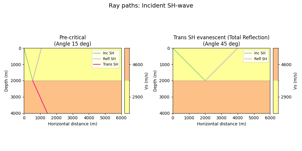
Ray diagrams (SH-incidence)

scenarios_sh = [
    (15, "Pre-critical"),
    (45, "Trans SH evanescent (Total Reflection)"),
]

fig, axes = plt.subplots(1, 2, figsize=(10, 5), sharey=True, sharex=True)

for i, (ang, name) in enumerate(scenarios_sh):
    plot_ray_situation(ang, "SH", name, axes[i])

show_ray_subplot_labels(axes)
fig.suptitle("Ray paths: Incident SH-wave", fontsize=14)
fig.tight_layout()
plt.show()

References

[1]

V. Červený. Seismic Ray Theory. Cambridge University Press, 2001. doi:10.1017/CBO9780511529399.

[2]

T. Lay and T. C. Wallace. Modern Global Seismology. Academic Press, 1995.