07.1 Magnitude sensitivity for homogeneous model: 1-km DAS array benchmark

This is an example of computing magnitude sensitivity for a homogeneous model.

It reproduces the homogeneous benchmark of a downhole DAS monitoring study: a 1-km-long vertical fibre with a constant noise level, used to isolate the effect of the DAS directional sensitivity before any velocity structure is introduced.

Test case 7:

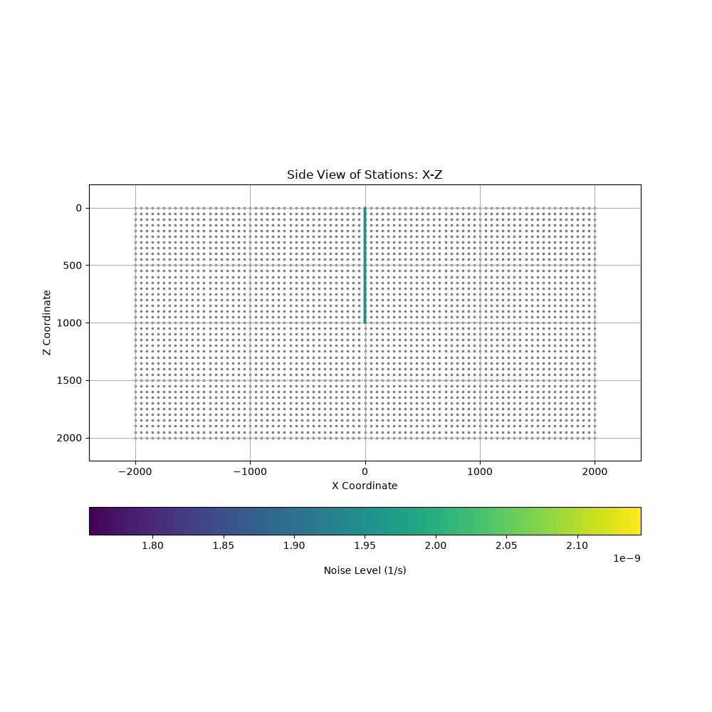
• Geometry: 1-km-long DAS cable in a vertical borehole, 1 m channel spacing, so 1000 channels between 1 m and 1000 m depth

• Data: constant strain-rate noise level of 1.95e-9 1/s on every channel, gauge length of 10 m

• Velocity model: homogeneous, Vp = 2370 m/s, Vp/Vs = 2 (so Vs = 1185 m/s), Qp = Qs = 100, rho = 2500 kg/m^3

• Processing: magnitude sensitivity on a vertical section through the well, requiring detection on at least 60 channels with a signal-to-noise ratio of at least 2, for P-waves, S-waves and both together.

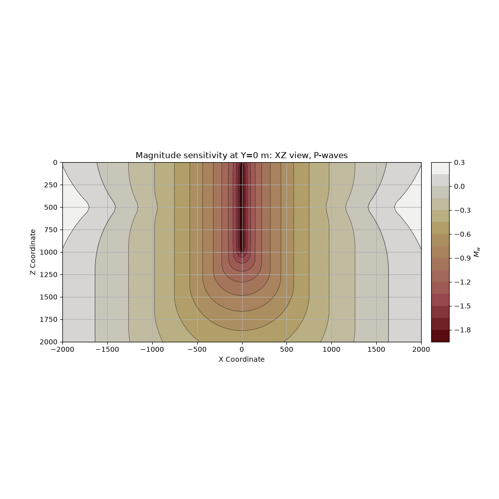
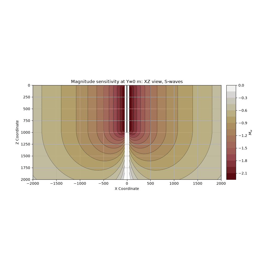
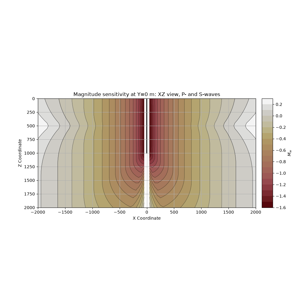
Three features of the resulting sections are worth looking for, and all three follow from the fact that a DAS cable only records the strain component along the fibre:

1. The minimum detectable magnitude grows with offset from the monitoring well.

2. P-wave sensitivity is worst near the mid-depth of the array, but only at offsets beyond half the array length, where the ray direction that a vertical fibre records best is no longer available anywhere along the cable.

3. S-wave sensitivity degrades below the array, and vanishes on the cable axis itself, where the S-wave polarization is perpendicular to the fibre.

Load all necessary packages

import pynetdesign.visualization as pndvis
import pynetdesign.modelling as pndmod
import numpy as np
from time import time

# sphinx_gallery_thumbnail_number = -1

Input

Read geometry

geometry_file_path = '../data/homo/test_07/TMPL_net_geometry_Noise_Constant.txt'
geometry_df = pndmod.io.read_geometry(geometry_file_path)

print(geometry_df)
print(geometry_df.attrs)

       Y    X       Z    NoiseLevel
0    0.0  0.0     1.0  1.950000e-09
1    0.0  0.0     2.0  1.950000e-09
2    0.0  0.0     3.0  1.950000e-09
3    0.0  0.0     4.0  1.950000e-09
4    0.0  0.0     5.0  1.950000e-09
..   ...  ...     ...           ...
995  0.0  0.0   996.0  1.950000e-09
996  0.0  0.0   997.0  1.950000e-09
997  0.0  0.0   998.0  1.950000e-09
998  0.0  0.0   999.0  1.950000e-09
999  0.0  0.0  1000.0  1.950000e-09

[1000 rows x 4 columns]
{'file_path': '../data/homo/test_07/TMPL_net_geometry_Noise_Constant.txt', 'original_coord_units': 'm', 'coordinate_system': 'local', 'noise_type': 'strain rate', 'noise_unit': '1/s', 'gauge_length': 10.0, '_is_combined': False}

Read velocity model

velocity_file_path = '../data/homo/test_07/TMPL_velocity_model.txt'
velocity_df = pndmod.io.read_velocity(velocity_file_path)

print(velocity_df)
print(velocity_df.attrs)

   Depth    Vp  VpVsRatio   Qp   Qs   Rho   Ep   Dt   Gm
0  40000  2370          2  100  100  2500  0.0  0.0  0.0
{'model_type': 'homo', 'model_anisotropy': 'isotropic', 'parameter_descriptions': {'Depth': 'Depth', 'Vp': 'P-wave velocity', 'Vs': 'S-wave velocity', 'VpVsRatio': 'Vp/Vs', 'Qp': 'P-wave quality factor', 'Qs': 'S-wave quality factor', 'Rho': 'density', 'Ep': 'Thomsen epsilon parameter', 'Dt': 'Thomsen delta parameter', 'Gm': 'Thomsen gamma parameter'}, 'parameter_units': {'Depth': 'm', 'Vp': 'm/s', 'Vs': 'm/s', 'VpVsRatio': '', 'Qp': '', 'Qs': '', 'Rho': 'kg/m^3', 'Ep': '', 'Dt': '', 'Gm': ''}}

Set imaging grid parameters

# Imaging grid parameters: a vertical section through the monitoring well,
# reaching twice the array length in offset and in depth
gx = np.arange(-2000, 2000 + 50, 50)
gy = np.array([0])
gz = np.arange(0, 2000 + 50, 50)

# Generate grid points
grid_points = pndmod.utils.generate_grid(x=gx, y=gy, z=gz)
print("Number of grid points:", grid_points.size)
print("Number of grid points in x:", gx.size)
print("Number of grid points in z:", gz.size)
print("grid_points.shape:", grid_points.shape)

Number of grid points: 9963
Number of grid points in x: 81
Number of grid points in z: 41
grid_points.shape: (3321, 3)

Plot geometry and imaging grid

_ = pndvis.geometry.plot_stations_view(geometry_df,
                                       view='xz',
                                       grid_points=grid_points,
                                       grid_marker_size=1,
                                       plot_names=False,
                                       station_marker_size=2)

Prepare to compute magnitude sensitivity

# Get medium parameters
density = velocity_df.at[0, 'Rho']
v_p = velocity_df.at[0, 'Vp']
Q_p = velocity_df.at[0, 'Qp']
v_s = velocity_df.at[0, 'Vp']/velocity_df.at[0, 'VpVsRatio']
Q_s = velocity_df.at[0, 'Qs']
print("density, v_p, Q_p, v_s, Q_s:", density, v_p, Q_p, v_s, Q_s)

# Minimum S/N for detection on an individual channel
min_SNR_p = 2
min_SNR_s = 2

# Minimum channels on which an event must be detected
min_stations_p = 60
min_stations_s = 60

# Save parameters. The source frequency is left unset, so that the representative
# frequency is the peak frequency of each arrival, clamped at the corner frequency
# of 100 Hz. The free surface correction is switched off: every channel of this
# cable is downhole, so none of them sees the doubling of a surface receiver.
params = pndmod.classes.DetectionParameters(
    min_SNR_p=min_SNR_p,
    min_SNR_s=min_SNR_s,
    min_stations_p=min_stations_p,
    min_stations_s=min_stations_s,
    fs_mode='off',
)

# Define the slice to use
slice_Y = 0

# Get the slice plane
Y_plane_points, Y_plane_indices = pndmod.utils.get_slice_coordinates(grid_points=grid_points,
                                                                     slice_dimension=1,
                                                                     slice_coordinate=slice_Y)

density, v_p, Q_p, v_s, Q_s: 2500 2370 100 1185.0 100

Compute magnitude sensitivity

print("Computing magnitude sensitivity...")

start_time = time()
Y_slice_mag_sens_p = pndmod.core.get_mag_sensitivity(grid_coords=Y_plane_points,
                                                     geometry_df=geometry_df,
                                                     velocity_df=velocity_df,
                                                     params=params,
                                                     wave_mode='P')
Y_slice_mag_sens_s = pndmod.core.get_mag_sensitivity(grid_coords=Y_plane_points,
                                                     geometry_df=geometry_df,
                                                     velocity_df=velocity_df,
                                                     params=params,
                                                     wave_mode='S')
Y_slice_mag_sens_ps = pndmod.core.get_mag_sensitivity(grid_coords=Y_plane_points,
                                                      geometry_df=geometry_df,
                                                      velocity_df=velocity_df,
                                                      params=params,
                                                      wave_mode='PS')
end_time = time()
print(f"Computation time: {end_time - start_time} seconds")

Computing magnitude sensitivity...
Computation time: 3.6952273845672607 seconds

Plot magnitude sensitivity

The three panels correspond to the three panels of the benchmark figure: P-waves only, S-waves only, and detection of both.

station_marker_size = 2
clb_range = None
plt_levels = None

Plot magnitude sensitivity for P wave

The sensitivity is worst at the mid-depth of the array, and that loss only appears at offsets larger than half the array length.

_ = pndvis.sensitivity.plot_sensitivity_slice(sens_data=Y_slice_mag_sens_p, xi=gx, zi=gz,
                                              plot_title=f"Magnitude sensitivity at Y={slice_Y} m: XZ view, P-waves",
                                              clb_title="$M_w$",
                                              geometry_df=geometry_df,
                                              plot_names=False,
                                              station_marker_size=station_marker_size,
                                              clb_range=clb_range,
                                              plt_levels=plt_levels)

Plot magnitude sensitivity for S wave

The S-wave polarization is perpendicular to the fibre on the cable axis, so the cable cannot record an S-wave arriving from directly below it.

_ = pndvis.sensitivity.plot_sensitivity_slice(sens_data=Y_slice_mag_sens_s, xi=gx, zi=gz,
                                              plot_title=f"Magnitude sensitivity at Y={slice_Y} m: XZ view, S-waves",
                                              clb_title="$M_w$",
                                              geometry_df=geometry_df,
                                              plot_names=False,
                                              station_marker_size=station_marker_size,
                                              clb_range=clb_range,
                                              plt_levels=plt_levels)

Plot magnitude sensitivity for P and S waves

Requiring both phases takes the worse of the two, so this panel inherits the P-wave loss at mid-depth and the S-wave loss below the array.

_ = pndvis.sensitivity.plot_sensitivity_slice(sens_data=Y_slice_mag_sens_ps, xi=gx, zi=gz,
                                              plot_title=f"Magnitude sensitivity at Y={slice_Y} m: XZ view, P- and S-waves",
                                              clb_title="$M_w$",
                                              geometry_df=geometry_df,
                                              plot_names=False,
                                              station_marker_size=station_marker_size,
                                              clb_range=clb_range,
                                              plt_levels=plt_levels)